Air Blower Sizing (Metric Units)

Summary

The objective of this example is to size a blower for an air distribution system, and evaluate the effect of different blower efficiencies on the blower size.

Topics Covered

• Sizing a Blower

• Changing Compressor Efficiencies

• Using Design Factors

• Using Scenario Manager

Required Knowledge

This example assumes the user has already worked through the Beginner: Air Heating System example, or has a level of knowledge consistent with that topic.  You can also watch the AFT Arrow Quick Start Video (English Units) on the AFT website, as it covers the majority of the topics discussed in the Beginner: Air Heating System example.

Model File

This example uses the following file, which is installed in the Examples folder as part of the AFT Arrow installation:

• US - Air Blower Sizing.aro

Problem Statement

An air distribution system requires a new blower. All of the pipes in the system are STD (schedule 40) steel, with adiabatic flow. You are to use a design factor of 1.1 on all of the pipe and junction friction losses. You can neglect elevation changes, and any losses at the branches. All of the pipes leading to the discharge rooms discharge at atmospheric pressure.

Use Redlich-Kwong for the equation of state model, and Generalized for the enthalpy model.

For the blower, there are three compression process cases to be examined:

• Adiabatic

• Efficiency = 80 Percent (set as Nominal Efficiency)

• Efficiency = 60 Percent

For these three cases, determine:

• The size of the blower for both flow and pressure rise to deliver a minimum of 250 scfm to each room.

• How the different compression process models for the blower affect the blower sizing and the discharge temperatures.

Step 1. Start AFT Arrow

From the Start Menu choose the AFT Arrow 9 folder and select AFT Arrow 9.

To ensure that your results are the same as those presented in this documentation, this example should be run using all default AFT Arrow settings, unless you are specifically instructed to do otherwise.

Step 2. Define the Fluid Properties Group

1. Open Analysis Setup from the toolbar or from the Analysis menu

2. Open the Fluid panel then define the fluid:

   1. Fluid Library = AFT Standard

   2. Fluid = Air

      1. After selecting, click Add to Model

   3. Equation of State = Redlich-Kwong

   4. Enthalpy Model = Generalized

   5. Specific Heat Ratio Source = Library

Step 3. Define the Pipes and Junctions Group

At this point, the first two groups are completed in Analysis Setup. The next undefined group is the Pipes and Junctions group. To define this group, the model needs to be assembled with all pipes and junctions fully defined. Click OK to save and exit Analysis Setup then assemble the model on the workspace as shown in the figure below.

The system is in place but now we need to enter the properties of the objects. Double-click each pipe and junction and enter the following properties.

Pipe Properties

1. Pipe Model tab

   1. Pipe Material = Steel - ANSI

   2. Pipe Geometry = Cylindrical Pipe

   3. Size = Use table below

   4. Type = STD (schedule 40)

   5. Friction Model Data Set = Standard

   6. Lengths = Use table below

Pipe	Size (inch)	Length (feet)
1	6	40
2	6	100
3-5, 7-8	4	250
6	4	500
9-13	2	100

2. Optional tab

   1. Pipe Friction = 1.1

Junction Properties

For this example, we need to determine the correct flow through the compressor. Now we need to use our engineering judgment to take an initial guess at the flow rate through the compressor. Assume 1250 scfm to start:

1. J1 Tank

   1. Elevation = 0 feet

   2. Fluid = Air

   3. Pressure = 0 psig

   4. Temperature = 70 deg. F

2. J2 Compressor/Fan

   1. Elevation = 0 feet

   2. Compressor Type = Centrifugal Compressor

   3. Compressor Model = Sizing

   4. Compression Process Thermodynamics = Adiabatic

   5. Compressor Sizing Parameter = Mass Flow Rate

   6. Fixed Flow Rate = 1250 scfm

3. All Assigned Pressures

   1. Elevation = 0 feet

   2. Pressure Model tab

      1. Fluid = Air

      2. Pressure = 0 psig

      3. Temperature = 70 deg. F

      4. Pressure Specification = Stagnation

   3. Loss Coefficient tab

      1. K - Flow into pipe = 1

      2. K - Flow out of pipe = 1

   4. Optional tab

      1. Junction Friction Loss = 1.1

4. All Branches

   1. Elevation = 0 feet

ØTurn on Show Object Status from the View menu to verify if all data is entered. If so, the Pipes and Junctions group in Analysis Setup will have a check mark. If not, the uncompleted pipes or junctions will have their number shown in red. If this happens, go back to the uncompleted pipes or junctions and enter the missing data.

Step 4. Specify the Output Control

Open the Output Control window by selecting Output Control from the Toolbar or Tools menu.

Select the units scfm for the Mass Flow Rate parameter for both Pipes and Junctions output.

Step 5. Create Child Scenarios

Using the Scenario manager, create one child scenario named 1250 scfm then three child scenarios to that scenario for the air blower evaluation. Name the first Adiabatic, name the second 80% Efficient, and name the third 60% Efficient. For the compressor in each scenario, open the Compressor/Fan Properties window, and set the following:

1. For the Adiabatic case, no changes are necessary. The Compression Process Thermodynamics for the Compressor is already set to Adiabatic and no Nominal Efficiency is entered.

2. For the 80% Efficient case, set the Nominal Efficiency to 80 Percent, and set the Compression Process Thermodynamics to Determine From Efficiency Data.

3. For the 60% Efficient case, set the Nominal Efficiency to 60 Percent, and set the Compression Process Thermodynamics to Determine From Efficiency Data.

Step 6. Run the Models

Load the Adiabatic scenario and click Run Model on the toolbar or from the Analysis menu. This will open the Solution Progress window. This window allows you to watch as the AFT Arrow solver converges on the answer. This model runs very quickly. Now view the results by clicking the Output button at the bottom of the Solution Progress window.

Repeat this process for each of the three child scenarios.

Step 7. Examine the Output

The Output window contains all the data that was specified in the Output Control window. 

Based upon the initial flow rate guess for the blower of 1250 scfm, not all rooms are receiving a minimum flow rate of 250 scfm. Therefore, the flow rate at the blower must be increased until each room receives a minimum flow rate of 250 scfm.

Determining the required blower flow rate can be easily accomplished through manual iteration on the blower flow rate. In order to automate this process of iteration, the AFT Arrow Goal Seek and Control (GSC) add-on module can assist with this greatly.

Right-click the 1250 scfm scenario and select Clone with Children. Iterate the blower mass flow rate until the 250 scfm is achieved.

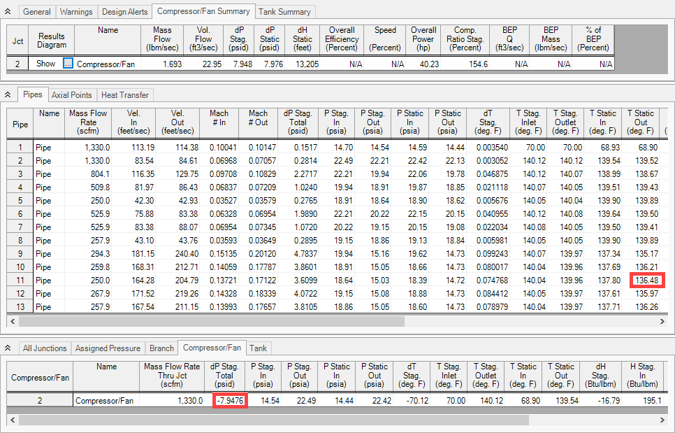
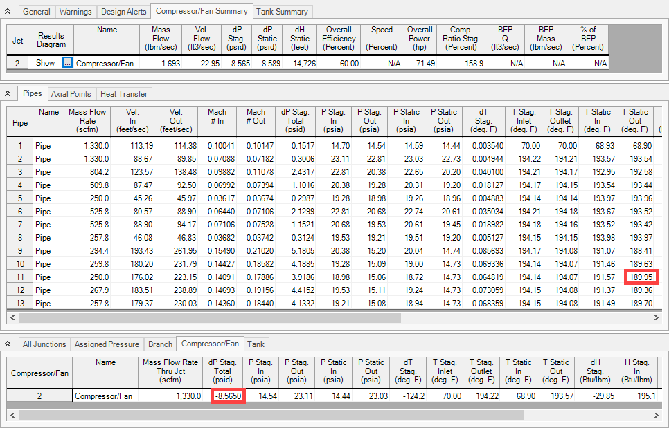
The output for each of the scenarios is shown in Figure 2, Figure 3, and Figure 4. This output is based upon the final required blower flow rate that will deliver a minimum flow rate of 250 scfm to each room.

The results are as follows:

Step 8. Evaluate 60% Efficiency with Heat Transfer

The engineers on the project have realized that the pipes are not insulated, and that the adiabatic assumption may be overly conservative. One engineer has also expressed concern that the discharge air could be too hot.

Create a child scenario to the 1330 scfm 60% efficient case named With Heat Transfer. Add heat transfer to the model on all the pipes by selecting Convective Heat Transfer as the Heat Transfer Model. For the Ambient Conditions, enter a Temperature of 80 deg. F, a Fluid Velocity of 7 miles/hr, and Air as the Fluid. See Figure 5 for this input.

Run the new scenario and determine the following:

• Do the compressor size requirements change significantly?

• How much do the discharge temperatures decrease?

Step 9. Examine the Output for 60% Efficiency with Heat Transfer

The output for this scenario is shown in Figure 6.

The blower stagnation pressure rise decreases from 8.5650 to 7.4769 psid, which is a 13% reduction. The max discharge temperature decreases to 88.47 deg. F.