Compressed Air System (Metric Units)

Summary

This example will demonstrate how to determine the range of outlet temperatures for a system given the range values for the system parameters.

Topics Covered

• Modeling Compressors with curve data

• Entering heat transfer data for pipes

• Using Scenarios

• Using the Copy Data From Jct... editing feature

Required Knowledge

This example assumes the user has already worked through the Beginner: Air Heating System example, or has a level of knowledge consistent with that topic.  You can also watch the AFT Arrow Quick Start Video (English Units) on the AFT website, as it covers the majority of the topics discussed in the Beginner: Air Heating System example.

Model File

This example uses the following file, which is installed in the Examples folder as part of the AFT Arrow installation:

• US - Compressed Air System.aro

Problem Statement

In this example, four machine tools are supplied air for operations. The machine tools are sensitive to temperature; therefore, the manufacturer needs to know the delivery temperature extremes the tools will see.

The air is taken from atmospheric conditions outside the building. Atmospheric pressure will remain constant at 0 psig, and the air temperature outside can vary from 0 to 110 deg. F. The temperature inside the building ranges from 70 to 75 deg. F.

The compressor used to drive the system has the following pressure characteristics:

• 12 psid at 0 lbm/sec 

• 10 psid at 0.5 lbm/sec

• 6 psid at 1 lbm/sec

The compressor efficiency is not known for certain, but it is expected to be between 80% and 90%.

The nozzles at the tools have a pressure drop of 8 psid at 0.2 lbm/sec. The nozzles discharge to atmospheric pressure.

The pipes in the system are uninsulated steel with an ambient air velocity that varies from 1 to 15 miles/hr. The pipe at the compressor inlet is heavily insulated (adiabatic). All of the components in the system are at an elevation of 0 feet.

What are the temperature extremes at the tools that this system could have?

Step 1. Start AFT Arrow

From the Start Menu choose the AFT Arrow 9 folder and select AFT Arrow 9.

To ensure that your results are the same as those presented in this documentation, this example should be run using all default AFT Arrow settings, unless you are specifically instructed to do otherwise.

Step 2. Define the Fluid Properties Group

1. Open Analysis Setup from the toolbar or from the Analysis menu

2. Open the Fluid panel then define the fluid:

   1. Fluid Library = AFT Standard

   2. Fluid = Air

      1. After selecting, click Add to Model

   3. Equation of State = Redlich-Kwong

   4. Enthalpy Model = Generalized

   5. Specific Heat Ratio Source = Library

Step 3. Define the Pipes and Junctions Group

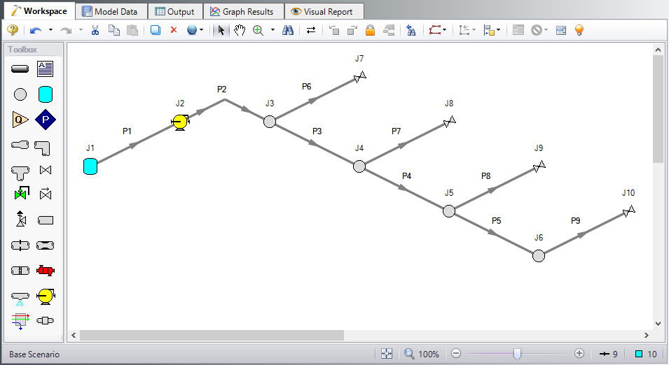
At this point, the first two groups are completed in Analysis Setup. The next undefined group is the Pipes and Junctions group. To define this group, the model needs to be assembled with all pipes and junctions fully defined. Click OK to save and exit Analysis Setup then assemble the model on the workspace as shown in the figure below.

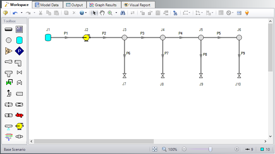
For this problem, you are required to determine the temperature extremes at the tools based on the range of system specifications. To do this, you will use the Scenario Manager to examine the hot and cold extremes for the system. 

The Scenario Manager is a powerful tool for managing variations of a model, referred to as scenarios.

The Scenario Manager allows you to:

• Create, name, and organize scenarios

• Select the scenario to appear in the Workspace (the ‘current’ scenario)

• Delete, clone, and rename scenarios

• Duplicate scenarios and save them as separate models

• Review the source of a scenario’s specifications

• Pass changes from a parent scenario to its child scenarios

The system is in place but now we need to enter the properties of the objects. Double-click each pipe and junction and enter the following properties. The Base Scenario will contain all of the basic model data for the system.

Pipe Properties

1. Pipe Model tab

   1. Pipe Material = Steel - ANSI

   2. Pipe Geometry = Cylindrical Pipe

   3. Size = Use table below

   4. Type = STD (schedule 40)

   5. Friction Model Data Set = Standard

   6. Lengths = Use table below

Pipe	Size	Length (feet)
1	2 inch	1
2-5	2 inch	25
6-9	1 inch	10

Junction Properties

1. J1 Tank

   1. Elevation = 0 feet

   2. Fluid = Air

   3. Pressure = 0 psig

   4. Temperature = 110 deg. F

2. J2 Compressor/Fan

   1. Elevation = 0 feet

   2. Model Type = Centrifugal Compressor

   3. Compressor Model = Compressor Curve

   4. Added Pressure = Stagnation

   5. Compression Process Thermodynamics = Determine From Efficiency Data

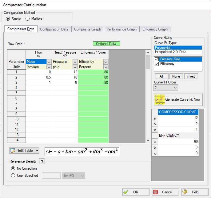
   6. Enter Curve Data =

Mass	Pressure	Efficiency
lbm/sec	psid	Percent
0	12	80
0.5	10	80
1	6	80

7. Curve Fit Order = 2

8. Click Generate Curve Fit Now

3. J3-J6 Branches

   1. Elevation = 0 feet

4. J7 Valve

   1. Elevation = 0 feet

   2. Valve Data Source = User Specified

   3. Subsonic Loss Model = Resistance Curve

   4. Exit Valve (optional) = Checked

   5. Exit Pressure = 0 psig

   6. Exit Temperature = 70 deg. F

   7. Enter Curve Data =

Mass	Pressure
lbm/sec	psid
0.2	8

8. Click Fill As Quadratic

9. Curve Fit Order = 2

10. Click Generate Curve Fit Now

5. J8-J10 Valves

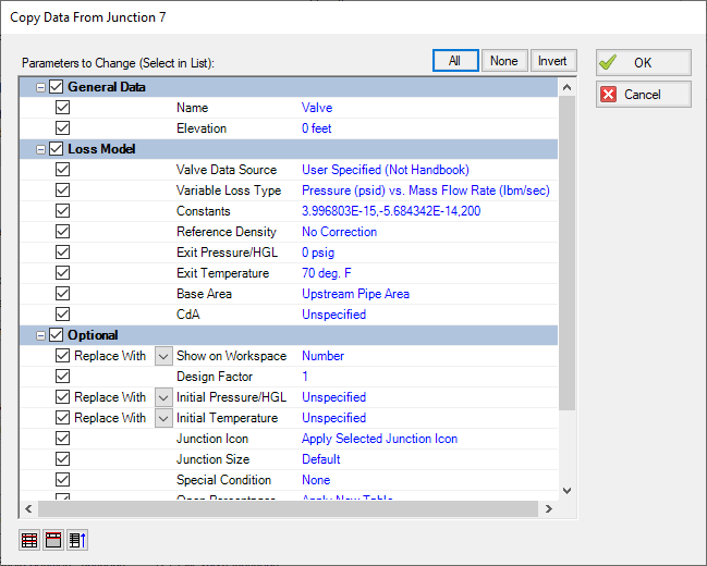
   1. Open the Valve Property window, and in the Copy Data From Jct drop-down list at the top, select J7. This will open the Copy Data From Junction window. Click All at the top. This will cause all of the properties to be set to the same as the properties for J7 (see Figure 3). Click OK. J8 now has all of the same properties as J7.

   2. Repeat this process for J9 and J10.

ØTurn on Show Object Status from the View menu to verify if all data is entered. If so, the Pipes and Junctions group in Analysis Setup will have a check mark. If not, the uncompleted pipes or junctions will have their number shown in red. If this happens, go back to the uncompleted pipes or junctions and enter the missing data.

Step 4. Create the Scenarios

Now you will use the Scenario Manager on the Quick Access Panel to create our temperature extreme scenarios. Note that you can also use the Scenario Manager from the Tools menu if you prefer.

From the Quick Access Panel, either right click on the Base Scenario and select Create Child, or select the Create Child icon .  Enter the name Hot Case in the Create Child Scenario window, as shown in Figure 4. Then click OK.

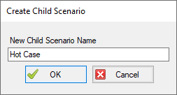
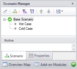
Select the Base Scenario in the Quick Access Panel, and then create another child. Enter the name Cold Case in the Create Child Scenario window and click OK. The Scenario Manager on the Quick Access Panel should now show two child scenarios below the Base Scenario, as shown in Figure 5.

Step 5. Modify the Hot Case Scenario

Double-click on the Hot Case scenario in the Quick Access Panel to load the Hot Case scenario. Alternatively, you can select the Hot Case scenario from the Quick Access Panel and then click on the Load Scenario icon to load the scenario.

In order to simulate the Hot Case such that the tools would experience the highest temperatures, you must assume the highest inlet and ambient temperatures as well as the worst heat transfer properties of the piping and lowest compressor efficiency. Make these changes to the following pipes:

1. P2-P9 Pipes

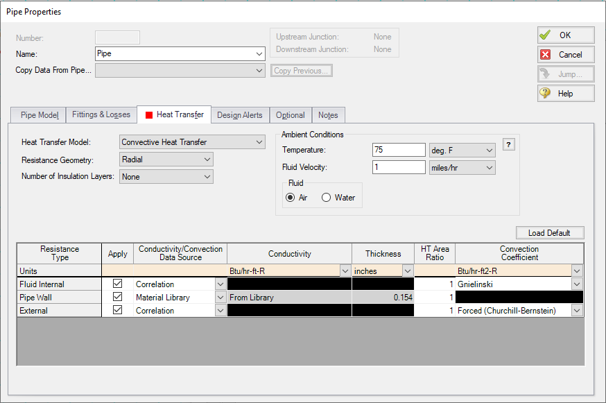
   1. The heat transfer properties of the uninsulated pipes should be set to the values as shown in Figure 6 (the wall thickness for the Pipe Wall will vary, depending on the diameter of the pipe). Change the Heat Transfer Model to Convective Heat Transfer. Next, enter a Temperature of 75 deg. F and enter a Fluid Velocity of 1 miles/hr. Doing so will minimize the heat transfer occurring in the pipe, and result in the highest temperature at the tools. Use the Global Pipe Edit tool to define the heat transfer information for all pipes at once.

Step 6. Run the Model

Click Run Model on the toolbar or from the Analysis menu. This will open the Solution Progress window. This window allows you to watch as the AFT Arrow solver converges on the answer. Once the solver has converged, view the results by clicking the Output button at the bottom of the Solution Progress window.

Step 7. Examine the Output

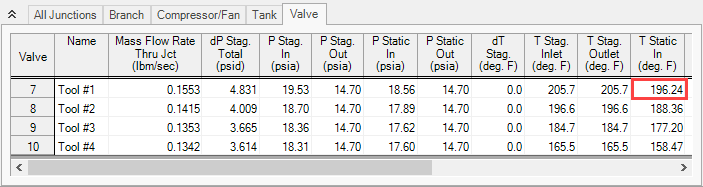
The Output window contains all the data that was specified in the Output Control window. The output for the Hot Case Scenario is shown in Figure 7. The valve output window shows the highest static temperature at the tools for the Hot Case is 196.24 deg. F at Tool 1 (T Static In).

Step 8. Modify the Cold Case Scenario

Open the Scenario Manager again from the Tools menu (or use the Scenario Manager in the Quick Access Panel). Select the Cold Case scenario in the Scenario Manager, and then click Load As Current Scenario to open the Cold Case scenario.

In order to simulate the Cold Case such that the tools would experience the lowest temperatures, you must assume the lowest inlet and ambient temperatures as well as the best heat transfer properties of the piping and highest compressor efficiency. Make these changes to the following objects:

1. J1 Tank

   1. Temperature = 0 deg. F

2. J2 Compressor

   1. The compressor will generate less heat if it is more efficient. Since this is the lower temperature case, you must assume the best feasible efficiency, which is 90%. This data is entered in the Compressor/Fan Configuration window. Since you used 80% in the table when you added the compressor information in the Base Scenario (Step 6), change the efficiency in the Raw Data table to 90%, and then click Generate Curve Fit Now to generate a new compressor curve.

3. Pipes P2-P9

   1. Set the heat transfer properties of the uninsulated pipes after the compressor to the values that will result in the lowest gas temperatures at the tools. The appropriate ambient temperature to use is the lowest of 70 deg. F. However, it is not clear which convection coefficient should be used. If the heat of compression at the compressor heats the gas to a temperature higher than 70 deg. F, we should use the highest ambient air velocity of 15 miles/hr. This will permit maximum cooling of the gas in the pipe. On the other hand, if the compressor discharge temperature is less than 70 deg. F, then the lowest ambient air velocity of 1 miles/hr should be used. This will yield the least heating of the gas in the pipes, giving the lowest possible temperature at the tools. Here we will use the value of 15 miles/hr. As just discussed, in practice one would need to verify the validity of this assumption.

Step 9. Run the Model

Click Run Model on the toolbar or from the Analysis menu. This will open the Solution Progress window. This window allows you to watch as the AFT Arrow solver converges on the answer. Once the solver has converged, view the results by clicking the Output button at the bottom of the Solution Progress window.

Step 10. Examine the Output

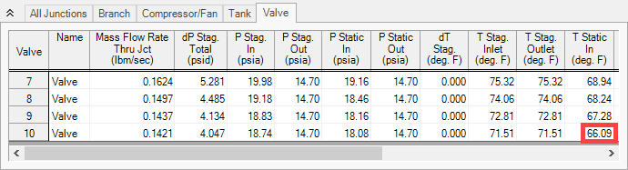
The Output window contains all the data that was specified in the Output Control window. The output for the Cold Case Scenario is shown in Figure 8. The valve output window shows the lowest static temperature at the tools for the Cool Case is 66.09 deg. F at Tool 4 (Tstatic In).

Note that the compressor discharge stagnation temperature is 77.95 deg. F, and thus the assumption of 15 mph for the ambient air velocity was appropriate.

Step 11. Use the Isometric Grid

AFT Arrow allows the user to place pipe or junction objects anywhere in the Workspace. Objects are placed on a 2D grid by default, as was the case with this example. At times it may be convenient to demonstrate the three-dimensional nature of a system. For example, if you are building a model based on isometric reference drawings. AFT Arrow includes an Isometric Pipe Drawing Mode for these cases. The isometric grid has three gridlines that are offset by 60°, representing the x, y, and z axes. Figure 9 shows the compressed air system built on an isometric grid.

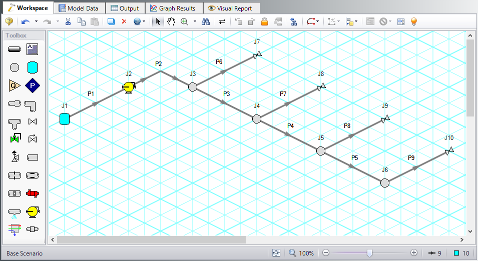
You can enable the isometric grid by going to the Arrange menu. Under Pipe Drawing Mode, there are three options: 2D Freeform (default), 2D Orthogonal, and Isometric.

Creating the compressed air system on an isometric grid will demonstrate how to use this feature.

1. Go to the File menu and select New.

2. From the Arrange menu, Show Grid and choose Isometric under Pipe Drawing Mode.

3. Place junctions J1-J7 on the Workspace in the positions shown in Figure 9.

4. You will notice that placing junctions onto the Workspace follows the usual rules, however, the visual appearance of the icons can be more complex than on a 2D grid. Due to the increased number of axes, the preferred icon and rotation can be selected to obtain visual consistency. Right click on J7 and select Customize Icon. Click the Rotate button and select the icon shown in Figure 10.

5. Copy J7 for the tools, J8-J10, to maintain the preferred icon.

6. Draw P1, as shown in Figure 11

7. Draw P2 from J2 to J3. A red-dashed preview line will show how the pipe will be drawn on the isometric grid. As you are drawing a pipe, you can change the preview line by clicking any arrow key on your keyboard or scrolling the scroll wheel on your mouse. Figure 11 shows Pipe 2 being drawn with the preview line.

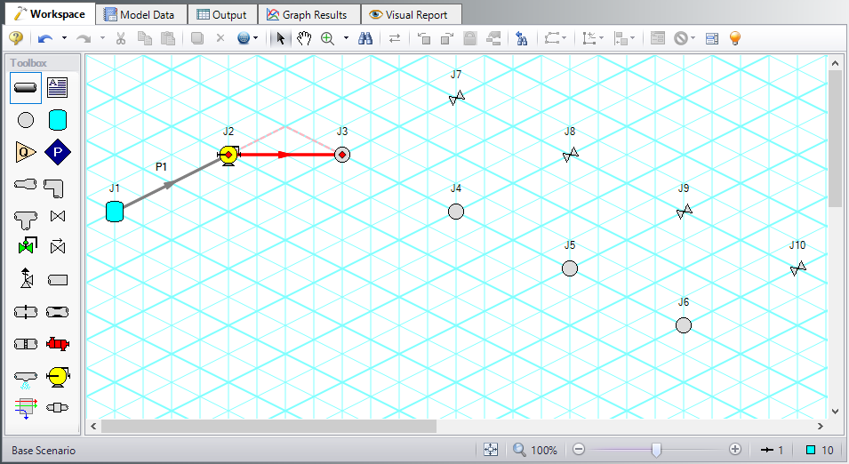
Note: You can hold the ALT key while adjusting a pipe by the endpoint to add an additional segment. This can be used with the arrow key or mouse scroll wheel to change between different preview line options.

8. Draw pipes P3-P9, as shown in Figure 12.

9. The grid can be shown or turned off in the Arrange menu.

Conclusion

By carefully selecting the input parameters from the specified system parameters, you were able to use AFT Arrow to determine the temperature extremes of the gas being supplied to the tools in the compressed air system. This information can now be sent to the tool manufacturer, who will use it to compensate for the temperature sensitivity of the tools.