Control Valve (Metric Units)

Summary

This example will walk you through a simple calculation to calculate a pipe size for a system with a control valve.

Topics Covered

• Using flow control valves

• Entering and changing pipe size data

• Adding items to the output using Output Control

• Modifying output using Output Control

Required Knowledge

This example assumes the user has already worked through the Beginner: Air Heating System example, or has a level of knowledge consistent with that topic.  You can also watch the AFT Arrow Quick Start Video (English Units) on the AFT website, as it covers the majority of the topics discussed in the Beginner: Air Heating System example.

Model File

This example uses the following file, which is installed in the Examples folder as part of the AFT Arrow installation:

• US - Control Valve.aro

Problem Statement

For this problem, steam flows from one tank to another. The pipe between the tanks is horizontal, and 450 feet long. A control valve is used to control the flow. The control valve must have a pressure drop of at least 20 psid to operate correctly. Assume the control valve is in the middle of the pipe. The ambient temperature is 60 deg. F. The pipe has an ambient air velocity of 15 miles/hr, and no insulation. The inlet stagnation pressure and temperature values are 240 psig and 425 deg. F, and the outlet stagnation pressure and temperature values are 140 psig and 425 deg. F. Note that the discharge temperature does not have an impact on calculations unless the discharge boundary happens to be supplying flow. Therefore, an assumed temperature can be used.

The pipe must be sized correctly to allow 5 lbm/sec to flow from one reservoir to the other. Consider only STD (schedule 40) pipes.

Step 1. Start AFT Arrow

From the Start Menu choose the AFT Arrow 9 folder and select AFT Arrow 9.

To ensure that your results are the same as those presented in this documentation, this example should be run using all default AFT Arrow settings, unless you are specifically instructed to do otherwise.

Step 2. Define the Fluid Properties Group

1. Navigate to the Fluid panel in Analysis Setup

2. Define the Fluid panel with the following inputs

   1. Fluid Library = AFT Standard

   2. Fluid = Steam

      1. After selecting, click Add to Model

   3. Equation of State = Redlich-Kwong

   4. Enthalpy Model = Generalized

   5. Specific Heat Ratio Source = Library

Step 3. Define the Pipes and Junctions Group

At this point, the first two groups are completed in Analysis Setup. The next undefined group is the Pipes and Junctions group. To define this group, the model needs to be assembled with all pipes and junctions fully defined. Click OK to save and exit Analysis Setup then assemble the model on the workspace as shown in the figure below.

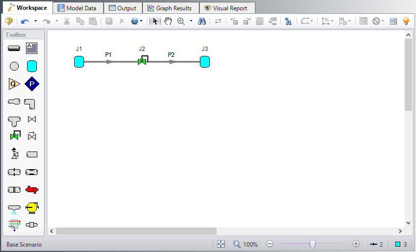
The system is in place but now we need to enter the properties of the objects. Double-click each pipe and junction and enter the following properties.

For this example, you need to find the correct pipe size but you are limited to STD (schedule 40) pipe sizes. You need to use your engineering judgment to take an initial guess at the pipe size for 5 lbm/sec. Try 2-½ inch pipe. Specify the pipes as follows:

Pipe Properties

1. Pipe Model tab

   1. Pipe Material = Steel - ANSI

   2. Pipe Geometry = Cylindrical Pipe

   3. Size = 2-1/2 inch

   4. Type = STD (schedule 40)

   5. Friction Model Data Set = Standard

   6. Length = 225 feet

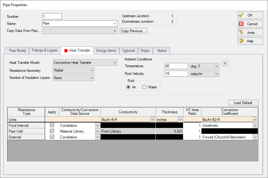
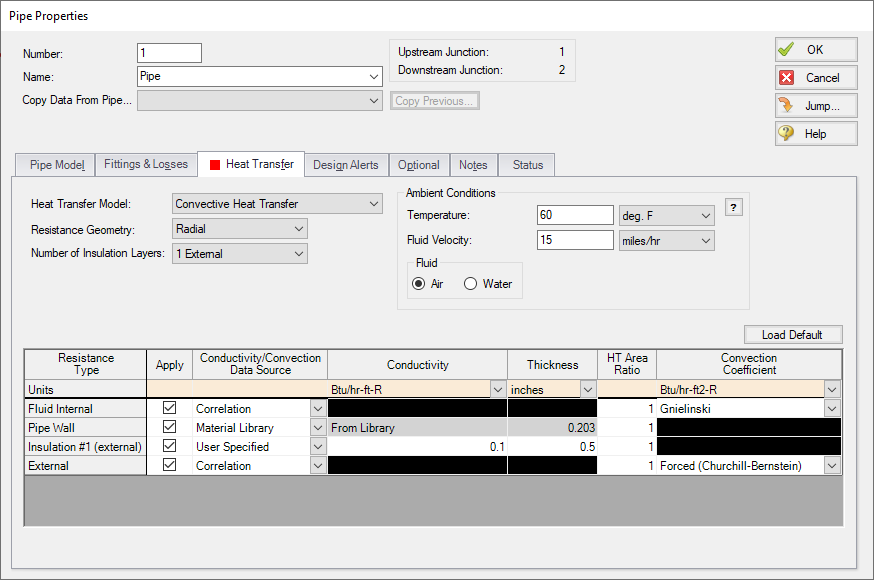
2. Heat Transfer tab

   1. Heat Transfer Model = Convective Heat Transfer

   2. Temperature = 60 deg. F

   3. Fluid Velocity = 15 miles/hr

   4. Fluid = Air

Junction Properties

1. J1 Tank

   1. Elevation = 0 feet

   2. Fluid = Steam

   3. Pressure = 240 psig

   4. Temperature = 425 deg. F

2. J2 Control Valve

   1. Elevation = 0 feet

   2. Valve Type = Flow Control (FCV)

   3. Control Setpoint = Mass Flow Rate

   4. Flow Setpoint = 5 lbm/sec

   5. Always Control (Never Fail) = Unchecked

3. J3 Tank

   1. Elevation = 0 feet

   2. Fluid = Steam

   3. Pressure = 140 psig

   4. Temperature = 425 deg. F

ØTurn on Show Object Status from the View menu to verify if all data is entered. If so, the Pipes and Junctions group in Analysis Setup will have a check mark. If not, the uncompleted pipes or junctions will have their number shown in red. If this happens, go back to the uncompleted pipes or junctions and enter the missing data.

Step 4. Run the Model

Click Run Model on the toolbar or from the Analysis menu. This will open the Solution Progress window. This window allows you to watch as the AFT Arrow solver converges on the answer. Once the solver has converged, view the results by clicking the Output button at the bottom of the Solution Progress window.

Step 5. Specify the Output Control

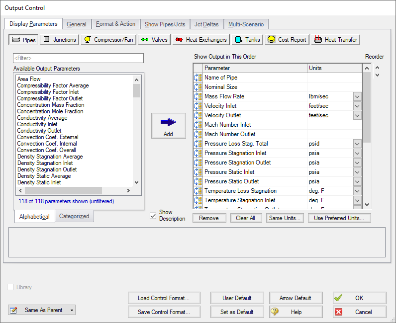
Open the Output Control window by selecting Output Control from the Toolbar or Tools menu.

In this example, you want to review the effects of changing the pipe nominal size. To simplify this, add this parameter to the output.

1. Click the Pipes button in the Display Parameters tab.

2. In the list on the left, find the parameter Nominal Size.

3. Select the Nominal Size parameter and then click the Add button, which adds the parameter to the list of displayed parameters on the right.

4. Use the Reorder buttons (in the upper right) to move the Nominal Size up so that it becomes the second parameter in the list (see Figure 3).

5. Click OK.

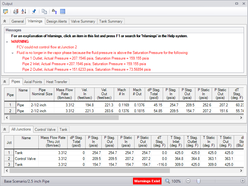
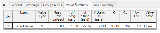
Step 6. Examine the Output

The Output window contains all the data that was specified in the Output Control window. The output is shown in Figure 4. In the General section of the Output window, there is a Warnings tab. Select this tab and you can see that for this case, the flow control valve was not able to achieve the required flow rate of 5 lbm/sec. The pressure drop across the valve is higher than the pressure drop required for the system to balance, so the valve is unable to maintain control for this size of pipe.

In addition warnings are shown that the fluid is above the saturation pressure line. AFT Arrow cannot calculate the actual behavior of the gas when the saturation line is reached. Instead Arrow will extrapolate the fluid properties assuming that the fluid would remain in the gas phase, and will warn the user that the saturation line was exceeded as is seen here.

Step 7. Size Piping Insulation

It is necessary to evaluate a new pipe size and to address the condensation warnings. Let's first address the condensation warnings, the pipe size will be addressed in the next step. We will assume that the necessary insulation thickness will not vary largely with pipe size because the expected change in pipe size should be relatively small in the next step.

One way to keep the fluid temperature above saturation and prevent condensation, would be to add insulation to the pipe. Assume there are three sizes of insulation available, 0.25 inch, 0.5 inch, and 1.0 inch thick, each of which has a thermal conductivity of 0.1 Btu/hr-ft-R. Assuming the same insulation for both pipes, which insulation size would be necessary to prevent condensation in the line?

Because this 2-1/2 inch model is valuable to refer to, keep this scenario by returning to the Workspace and then creating a new scenario on the Scenario Manager as a Child scenario by right-clicking on the Base Scenario and selecting Create Child. Name the child scenario With Insulation. Insulation is added on the Pipe Properties window's Heat Transfer tab. AFT Arrow allows you to specify up to three layers of insulation. The insulation can be specified as internal insulation, external insulation, or a combination of the two. Add the insulation to the pipe by changing the Number of Insulation Layers to 1 External, and then add the insulation thermal data to the table (see Figure 5). For Conductivity, enter 0.1 Btu/hr-ft-R and for thickness, enter 0.5 inches as an initial guess. Make these changes to both pipes.

Step 8. Change Pipe Size

Create a child scenario of the With Insulation scenario and name it 3 inch Pipe. From this scenario, select a new pipe size in the Pipe Properties window for both pipes. By trial and error, you can determine that by using 3-inch pipe, the minimum 20 psid pressure drop requirement can be satisfied (see Valve Summary tab in Figure 6). Do the results change if the valve is not in the middle of the pipe?

Conclusion

To meet the system requirements, 3-inch pipe should be used. If the valve were not in the middle of the pipe, the results would change because there is less pressure drop available as the valve is moved towards the pipe inlet. To prevent condensation in the line, the 0.5-inch thick insulation would have to be used.