Compressed Air System - Cost (English Units)
Compressed Air System - Cost Example (Metric Units)
Summary
This example demonstrates how to use the cost calculation features in AFT Arrow. All cost calculation features are included with Arrow.
Topics Covered
-
Estimating simple costs
-
Connecting cost libraries
-
Using Cost Settings
-
Using the Cost Report
Required Knowledge
This example assumes the user has already worked through the Beginner: Air Heating System example, or has a level of knowledge consistent with that topic. You can also watch the AFT Arrow
Model Files
This example uses the following files, which are installed in the Examples folder as part of the AFT Arrow installation:
-
Compressed Air System.dat - engineering library
-
Compressed Air System Costs.cst - cost library for Compressed Air System.dat
-
Steel - ANSI Pipe Costs.cst - cost library for Steel - ANSI
Problem Statement
Use the cost calculation features in AFT Arrow to determine the cost of the compressed air system over a 10-year period for both the hot and cold cases. Include material, installation, and energy costs.
Step 1. Start AFT Arrow
From the Start Menu choose the AFT Arrow 9 folder and select AFT Arrow 9.
To ensure that your results are the same as those presented in this documentation, this example should be run using all default AFT Arrow settings, unless you are specifically instructed to do otherwise.
Important: The GSC module and cost calculations can be used in the same run, but we are not going to do this here. Before proceeding, make sure to disable GSC by selecting the radio button for Ignore in the Modules panel in Analysis Setup.
Step 2. Define the Pipes and Junctions Group
Open the US - Compressed Air System.aro example file listed above, which is located in the Examples folder in the AFT Arrow application folder. Save the file to a different folder.
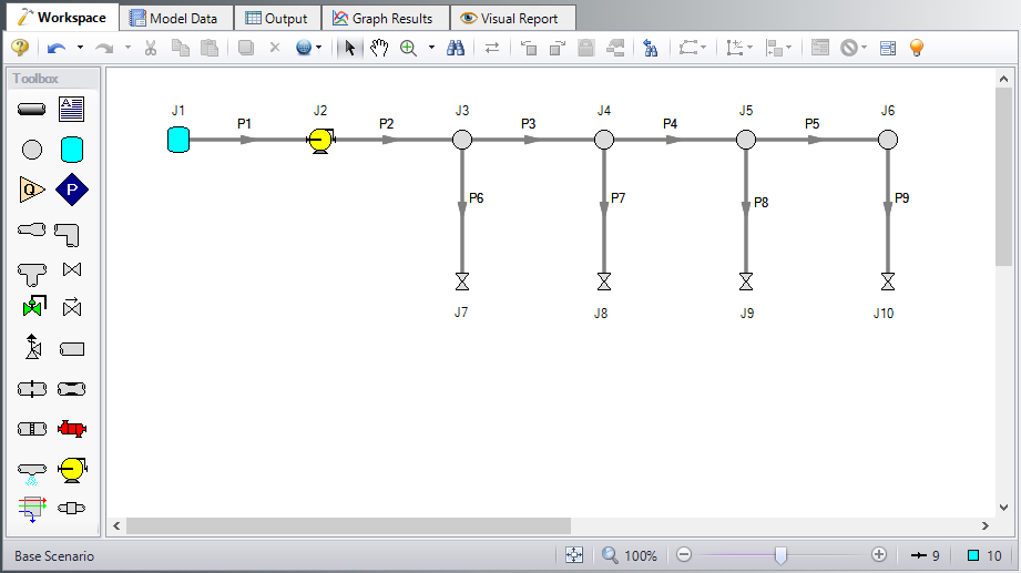
Once the model is opened and saved to a new location, load the Base Scenario. The workspace should look like Figure 1
Step 3. Define the Steady Solution Control Group
There is an option available in Solution Control when using one of the marching methods that can sometimes result in an overall reduction in solution runtime. This option is to first solve the system using the Lumped Adiabatic method and then use these results as a starting point for the marching solution. Since the Lumped Adiabatic solution can typically be obtained much faster, this can provide an overall reduction in runtime for the marching method.
The Steady Solution Control Group is already defined using the default inputs. This means that no user input is required to run the model. However, the Lumped Adiabatic initialization will be used for this model.
To activate this option, do the following:
-
Open Analysis Setup
-
Navigate to the Solution Method panel in the Steady Solution Control group
-
Click the box to turn on First Use Lumped Adiabatic Method To Obtain Initial Stating Point For Marching Solution
The Steady Solution Control Group is now defined for this model.
Step 4. Define the Cost Settings Group
To use the cost calculation feature, navigate to the Cost Settings panel in Analysis Setup.
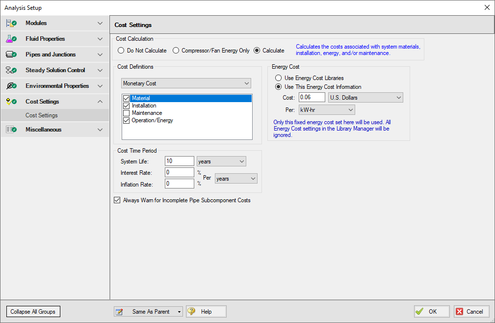
The Cost Settings panel is where the types of costs to be included in the cost calculations are specified. The Cost Settings panel is shown in Figure 2.
Energy cost data can be specified through an energy cost library, or by directly entering an energy cost in the Cost Settings window. Using an energy cost library allows you to specify multiple energy costs, such as energy costs at both peak and off-peak rates.
For this example, in the Cost Calculation section at the top, select Calculate. Next, in the Energy Cost section, enter an energy cost of 0.06 U.S. Dollars Per kW-hr, as shown in Figure 2.
The Cost Definitions section allows you to specify the type of costs to be determined. You may select from actual monetary costs, including Material, Installation, Maintenance, and Operation/Energy costs.
For this example, include Material, Installation, and Operation/Energy costs by selecting them from the list of available Monetary Costs, as shown in Figure 2.
The system lifetime to be applied for the cost calculations is specified in the Cost Time Period section. You can also specify interest and inflation rates to be applied to the cost calculations as well.
For this example, enter a System Life of 10 years, as shown in Figure 2, then close the Cost Settings window by clicking OK.
Step 5. Engineering and Cost Libraries
The actual material and installation costs that the cost calculation feature uses are contained in cost libraries. The cost libraries needed for this example already exist, and just need to be accessed.
The Library Manager (opened from the Library menu) shows all of the available and connected libraries. Libraries can either be engineering libraries or cost libraries. Cost libraries are always associated with an engineering library, and are thus displayed subordinate to an engineering library in the library lists.
Here we will summarize some key aspects of libraries:
-
Cost information for a pipe system component is accessed from a cost library. Cost library items are based on corresponding items in an engineering library. (The engineering libraries also include engineering information such as pipe diameters, hydraulic loss factors, etc.)
-
To access a cost for a particular pipe or junction in a model, that pipe or junction must be based on items in an engineering library. Moreover, that library must be connected.
-
There can be multiple cost libraries associated with and connected to an engineering library. This makes it easier to manage costs of items.
Add the Engineering and Cost Libraries
Select Library Manager from the Library menu. Add the Compressed Air System.dat engineering library file to the list of available libraries by clicking Add Existing Library at the bottom. Browse to the engineering library file in the AFT Arrow 9 Examples folder. The engineering library should now appear in the list of available libraries.
Now add the cost libraries by clicking Add Existing Cost, and browsing to the Compressed Air System Costs.cst and the Steel - ANSI Pipe Costs.cst cost library files.
All the added libraries should be connected automatically. If not connected, connect the newly added engineering libraries by selecting them in the list of available libraries, and clicking the Add to Connections button.
The Library Manager should appear as shown in Figure 3.
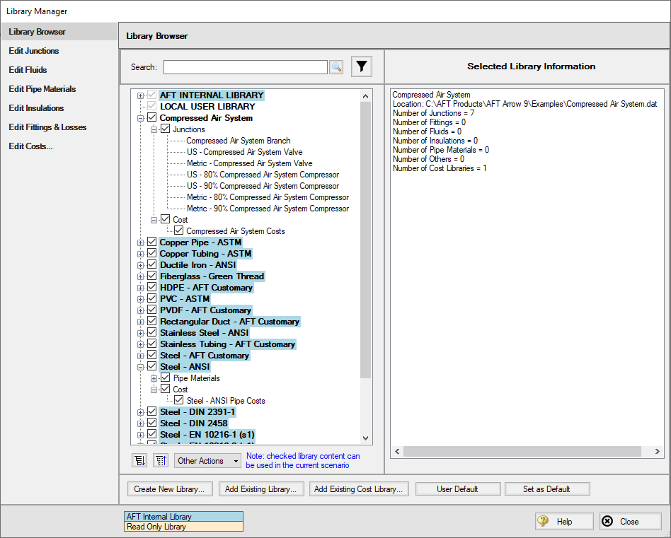
The engineering libraries associated with these two cost libraries are the Steel - ANSI pipe materials library, and an external library called Compressed Air System. For the cost data in the two cost libraries to be accessed by pipes and junctions in the model, the pipes and junctions must use these two engineering libraries.
The pipes for this example are already using data from the Steel - ANSI pipe material library, so no modifications need to be made for the pipes.
All of the junctions except the tank junction must be modified to use the component data contained in the engineering library. Do this by opening the Properties window for each junction, and selecting the component name displayed in the Library Jct list, as shown in Figure 4 for the Compressor/Fan junction.
Note that there are two compressor junctions in the library. One uses an efficiency of 80% for the Hot Case scenario, and the other uses an efficiency of 90% for the Cool Case scenario. For this case, select the
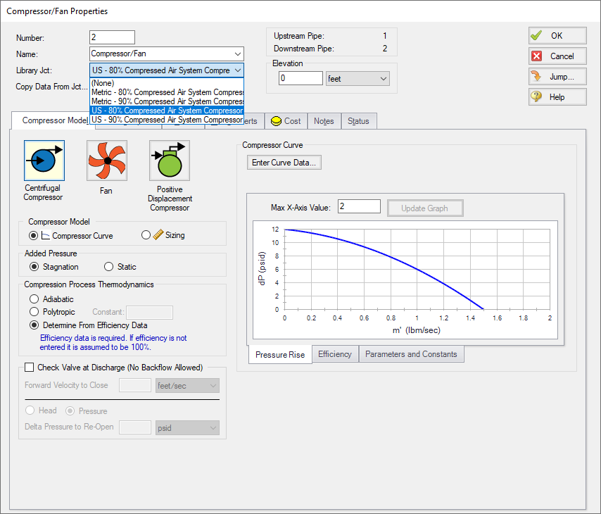
Figure 4: The components to be included in the cost analysis must be associated with an engineering library
Step 6. Include Cost in Report
The final step before performing a cost analysis is to specify which pipes and junctions you want to be included in the final cost report. This is done by choosing Include in Cost Report on the Cost tab in the Properties window for each pipe and junction to be included, as shown for Pipe 1 in Figure 5.
The Global Edit feature may be used to update this information for all of the pipes and junctions.
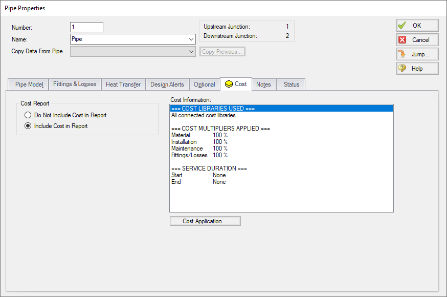
Figure 5: The Cost tabs on the pipe and junction Properties windows are used to include the objects in the Cost Report
Once all the necessary Pipes and Junctions have been set to be included in the Cost Report, load the Hot Case scenario.
Step 7. Run the Model
Click Run Model on the toolbar or from the Analysis menu. This will open the Solution Progress window. This window allows you to watch as the AFT Arrow solver converges on the answer. Once the solver has converged, view the results by clicking the Output button at the bottom of the Solution Progress window.
Step 8. Examine the Output
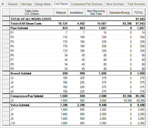
The Cost Report is displayed in the General section of the Output window. View the Cost Report by selecting the Cost Report tab. The content of the Cost Report can be controlled from the Output Control window. Figure 6 shows the Cost Report for this example with the Material, Installation, Operation, and Total costs displayed.
The Cost Report shows the total system cost, as well as the individual totals for the material, installation, and energy costs. In addition, the Cost Report displays the detailed cost for each pipe, junction, and fitting that was included in the report. The items are grouped together by type, and a subtotal for each category is listed.
Step 9. Set up and Run the Cold Case Scenario
Load the Cold Case scenario. Repeat Step 4 through Step 8 but using the
Cost Analysis Summary
The cost analysis for the Hot Case scenario shows that the total system cost over 10 years for the compressed air system is $97,943. Of that cost, $10,124 was for Material costs, $4,463 was for Installation costs, and $83,356 was energy cost over the life of the system.
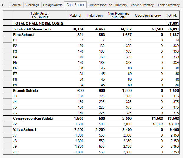
By contrast the cost analysis for the Cold Case scenario shows that the total system cost over 10 years for the compressed air system is $76,091. Of that cost, $10,124 was for Material costs, $4,463 was for Installation costs, and $61,503 was energy cost over the life of the system.


