Flow Through an Orifice (English Units)
Flow Through an Orifice (Metric Units)
Summary
This example demonstrates a sample calculation to determine the maximum flow through a system where sonic choking occurs, as well as the sonic pressure and area, and it explores the effect of CdA on the system flow rate.
Topics Covered
-
Determining the maximum flow through a system
-
Determining sonic (stagnation) pressure
-
Determining sonic area
-
Using scenarios
Required Knowledge
This example assumes the user has already worked through the Beginner: Air Heating System example, or has a level of knowledge consistent with that topic. You can also watch the AFT Arrow
Model File
This example uses the following file, which is installed in the Examples folder as part of the AFT Arrow installation:
Problem Statement
For this problem, steam flows from one tank to another, through an orifice.
The first pipe from the inlet tank to the orifice is
The inlet tank has a pressure of
The orifice at the end of the first pipe has an area of
Determine the following:
-
What is the maximum flow through the system?
-
What is the sonic (stagnation) pressure at the system exit?
-
At the maximum flow, what is the sonic area at the orifice? At the discharge tank?
Step 1. Start AFT Arrow
From the Start Menu choose the AFT Arrow 9 folder and select AFT Arrow 9.
To ensure that your results are the same as those presented in this documentation, this example should be run using all default AFT Arrow settings, unless you are specifically instructed to do otherwise.
Step 2. Define the Fluid Properties Group
-
Navigate to the Fluid panel in Analysis Setup
-
Define the Fluid panel with the following inputs
-
Fluid Library = AFT Standard
-
Fluid = Steam
-
After selecting, click Add to Model
-
-
Equation of State = Redlich-Kwong
-
Enthalpy Model = Generalized
-
Specific Heat Ratio Source = Library
-
Step 3. Define the Pipes and Junctions Group
At this point, the first two groups are completed in Analysis Setup. The next undefined group is the Pipes and Junctions group. To define this group, the model needs to be assembled with all pipes and junctions fully defined. Click OK to save and exit Analysis Setup then assemble the model on the workspace as shown in the figure below.
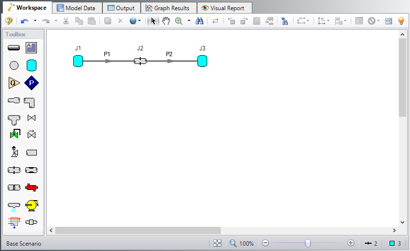
The system is in place but now we need to enter the properties of the objects. Double-click each pipe and junction and enter the following properties.
Pipe Properties
-
Pipe Model tab
-
Pipe Material = Steel - ANSI
-
Pipe Geometry = Cylindrical Pipe
-
Size = 2 inch
-
Type = STD (schedule 40)
-
Friction Model Data Set = Standard
-
Lengths =
-
| Pipe | Length (feet) |
|---|---|
| 1 | 10 |
| 2 | 20 |
Junction Properties
-
J1 Tank
-
Name = Inlet Tank
-
Elevation = 0 feet
-
Fluid = Steam
-
Pressure = 250 psig
-
Temperature = 500 deg. F
-
-
J2 Orifice
-
Elevation = 0 feet
-
Orifice Type = User Specified
-
Subsonic Loss Model = K Factor
-
Orifice Dimensions = Area
-
Area = 3 inches2
-
K = 10
-
-
J3 Tank
-
Name = Discharge Tank
-
Elevation = 0 feet
-
Fluid = Steam
-
Pressure = 0 psig
-
Temperature = 500 deg. F
-
ØTurn on Show Object Status from the View menu to verify if all data is entered. If so, the Pipes and Junctions group in Analysis Setup will have a check mark. If not, the uncompleted pipes or junctions will have their number shown in red. If this happens, go back to the uncompleted pipes or junctions and enter the missing data.
Step 4. Run the Model
Click Run Model on the toolbar or from the Analysis menu. This will open the Solution Progress window. This window allows you to watch as the AFT Arrow solver converges on the answer. Once the solver has converged, view the results by clicking the Output button at the bottom of the Solution Progress window.
Step 5. Specify the Output Control
Open the Output Control window by selecting Output Control from the Toolbar or Tools menu.
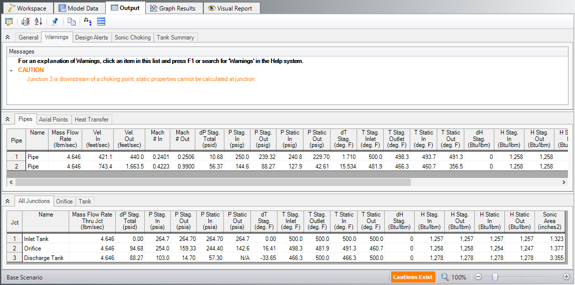
The Output window (Figure 2) contains all the data that is specified in the Output Control window. The window starts with a default set of outputs, which is normally sufficient. You can also specify the units for each output parameter from this window. For this example, change the Pressure Stagnation Inlet units to
Step 6. Examine the Output
Because this system chokes at the discharge tank, the Sonic Choking tab appears in the General section of the Output window. This tab will appear when sonic choking occurs in the system, and will contain messages pertaining to the sonic choking conditions.
Because the flow is choked at the exit, the mass flow rate shown in the Output reflects the maximum flow rate through the system for the given conditions. The maximum flow rate through this system is
Step 7. System Modification
Set the CdA (for Sonic Choking - Optional) in the Orifice Properties window to 20% higher than the sonic area and then 20% lower than the sonic area, and rerun the model for each scenario. How do the results change for each case?
Note: This is a situation where a user can create two new scenarios using the Scenario Manager to examine several what-if situations, without disturbing the basic model.
Step 8. Re-evaluate the Model
Setting the orifice CdA higher than the sonic area has no affect on the model because the system is already choking at the exit. Setting the CdA 20% lower than the sonic area


