Hydrocarbon Process Relief System (Metric Units)

Summary

This example will demonstrate how to determine the relief capacity of a system, where sonic choking occurs, and the pressure drop across a shock wave.

Topics Covered

• Understanding sonic choking

• Observing pressure drop across shock waves

• Using fluid mixtures

Required Knowledge

This example assumes the user has already worked through the Beginner: Air Heating System example, or has a level of knowledge consistent with that topic.  You can also watch the AFT Arrow Quick Start Video (English Units) on the AFT website, as it covers the majority of the topics discussed in the Beginner: Air Heating System example.

Model File

This example uses the following file, which is installed in the Examples folder as part of the AFT Arrow installation:

• US - Hydrocarbon Relief System.aro

Problem Statement

A mixture of 89% methane and 11% hydrogen (by mass) exists at a process facility. There is a plan to increase the process conditions to 935 psig at 100 deg. F. The relief system needs to be re-evalutated to determine if it will still be adequate under these conditions. Assume that all of the pipes are well insulated (i.e. adiabatic).

Determine the following:

• What is the relief capacity of the system under the new conditions?

• Where does sonic choking occur in the system, and why?

• What is the pressure drop across the shock wave(s)?

Step 1. Start AFT Arrow

From the Start Menu choose the AFT Arrow 9 folder and select AFT Arrow 9.

To ensure that your results are the same as those presented in this documentation, this example should be run using all default AFT Arrow settings, unless you are specifically instructed to do otherwise.

Step 2. Define the Fluid Properties Group

For this analysis, you will need to create and use a fluid mixture using the NIST REFPROP fluid library.

1. Open Analysis Setup from the toolbar or from the Analysis menu

2. Navigate to the Fluid panel

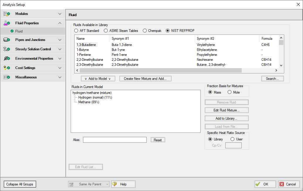
3. In the Fluids Available in Library section, select NIST REFPROP

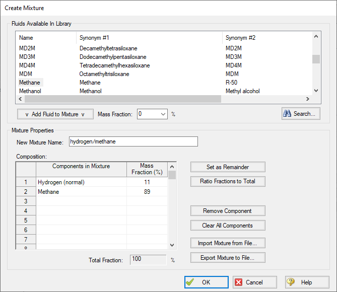
4. Click Create New Mixture and Add to open the Create Mixture window

5. Enter the name hydrogen/methane in the New Mixture Name field

6. Select Hydrogen (normal) from the list of Fluids Available In Library

7. Enter a Mass Fraction of 11% in the Mass Fraction field, then click Add Fluid to Mixture to add hydrogen to the list components in the mixture

8. Repeat this process for Methane, with a Mass Fraction of 89%

9. The Create Mixture window should now appear as shown in Figure 1

10. Click OK to add the mixture to the Fluids in Current Model on the Fluid panel, as shown in Figure 2

11. Ensure that Library is selected as the Specific Heat Ratio Source

Step 3. Define the Pipes and Junctions Group

At this point, the first two groups are completed in Analysis Setup. The next undefined group is the Pipes and Junctions group. To define this group, the model needs to be assembled with all pipes and junctions fully defined. Click OK to save and exit Analysis Setup then assemble the model on the workspace as shown in the figure below.

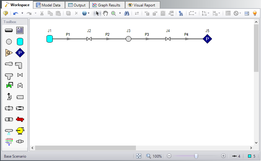
The system is in place but now we need to enter the properties of the objects. Double-click each pipe and junction and enter the following properties. Note the following:

• The Total K Factor listed for the pipes should be entered as the Total K Factor on the Fittings & Losses tab in the Pipe Properties window.

• The CdA values given for the valves are required for Sonic Choking calculations.

Pipe Properties

1. Pipe Model tab

   1. Pipe Material = Steel - ANSI

   2. Pipe Geometry = Cylindrical Pipe

   3. Size = Use table below

   4. Type = Use table below

   5. Friction Model Data Set = Standard

   6. Lengths = Use table below

   7. Total K Factor = Use table below

Pipe	Size (inch)	Type	Length (feet)	Total K Factor
1	6	STD (schedule 40)	24	4.4
2	6	STD (schedule 40)	21	4.2
3	10	STD (schedule 40)	25	2.1
4	16	STD (schedule 30)	258	8.9

Junction Properties

1. J1 Tank

   1. Name = Process

   2. Elevation = 12 feet

   3. Fluid = hydrogen/methane (mixture)

   4. Pressure = 935 psig

   5. Temperature = 100 deg. F

2. J2 Valve

   1. Name = Manual Valve

   2. Elevation = 6 feet

   3. Valve Data Source = User Specified

   4. Subsonic Loss Model = K Factor

   5. K = 10

   6. CdA (for Sonic Choking - optional) = 15 inches2

3. J3 Branch

   1. Name = Header Connection

   2. Elevation = 12 feet

4. J4 Valve

   1. Name = Relief Valve (assumed open)

   2. Elevation = 0 feet

   3. Valve Data Source = User Specified

   4. Subsonic Loss Model = K Factor

   5. K = 8.3

   6. CdA (for Sonic Choking - optional) = 45 inches2

5. J5 Assigned Pressure

   1. Name = Atmosphere

   2. Elevation = 22 feet

   3. Fluid = hydrogen/methane (mixture)

   4. Pressure = 0 psig

   5. Temperature = 100 deg. F

   6. Pressure Specification = Stagnation

ØTurn on Show Object Status from the View menu to verify if all data is entered. If so, the Pipes and Junctions group in Analysis Setup will have a check mark. If not, the uncompleted pipes or junctions will have their number shown in red. If this happens, go back to the uncompleted pipes or junctions and enter the missing data.

Step 4. Run the Model

Click Run Model on the toolbar or from the Analysis menu. This will open the Solution Progress window. This window allows you to watch as the AFT Arrow solver converges on the answer. Once the solver has converged, view the results by clicking the Output button at the bottom of the Solution Progress window.

Step 5. Specify the Output Control

Open the Output Control window by selecting Output Control from the Toolbar or Tools menu.

Set the units for Mass Flow to lbm/hr.

Step 6. Examine the Output

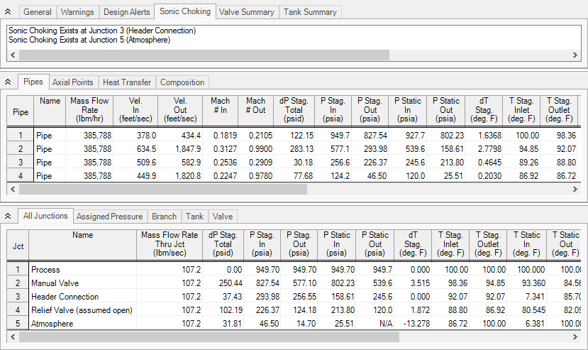
The output shows the capacity of the system is 383,788 lbm/hr, as shown in Figure 4.

The Sonic Choking tab in the General section of the Output window shows that the system chokes at J3, the Header Connection, and at J5, the discharge to atmosphere. The system chokes at J3 because of the expansion from 6-inch pipe to 10-inch pipe. The system chokes at J5 because of endpoint choking.

The pressure drop across the choke point is the same as the change in stagnation pressure. This can be seen in the Junction output section. The pressure drop across the choke point at J3 is 37.43 psid, and the pressure drop across the shock wave at J5 is 31.81 psid.