Process Steam System (English Units)
Process Steam System (Metric Units)
Summary
The objective of this example is to determine the minimum delivery pressure of a process steam supply system.
Topics Covered
-
Determining the minimum delivery pressure of a steam supply system.
-
Understanding Solution Control sensitivity
Required Knowledge
This example assumes the user has already worked through the Beginner: Air Heating System example, or has a level of knowledge consistent with that topic. You can also watch the AFT Arrow
Model File
This example uses the following file, which is installed in the Examples folder as part of the AFT Arrow installation:
Problem Statement
A process steam supply system has two boilers at
All of the pipes in the system have 2 inches of insulation with a thermal conductivity of 0.02 Btu/hr-ft-R, and an ambient air velocity of 7 mph. The ambient temperature is 75 deg. F. The pipes are all Steel - ANSI STD (schedule 40). All of the elbows in the system are Smooth, with an r/D of 1.5.
All of the tees in the system should be modeled using the Detailed loss model, with sharp edges.
The system has six users with the following peak flow demands:
-
40,000 lbm/hr
-
50,000 lbm/hr
-
60,000 lbm/hr
-
55,000 lbm/hr
-
40,000 lbm/hr
-
60,000 lbm/hr
Determine the following:
-
What is the minimum delivery (stagnation) pressure of the system, and at which user?
Step 1. Start AFT Arrow
From the Start Menu choose the AFT Arrow 9 folder and select AFT Arrow 9.
To ensure that your results are the same as those presented in this documentation, this example should be run using all default AFT Arrow settings, unless you are specifically instructed to do otherwise.
Step 2. Define the Fluid Properties Group
-
Navigate to the Fluid panel in Analysis Setup
-
Define the Fluid panel with the following inputs
-
Fluid Library = AFT Standard
-
Fluid = Steam
-
After selecting, click Add to Model
-
-
Equation of State = Redlich-Kwong
-
Enthalpy Model = Generalized
-
Specific Heat Ratio Source = Library
-
Step 3. Define the Pipes and Junctions Group
At this point, the first two groups are completed in Analysis Setup. The next undefined group is the Pipes and Junctions group. To define this group, the model needs to be assembled with all pipes and junctions fully defined. Click OK to save and exit Analysis Setup then assemble the model on the workspace as shown in the figure below.
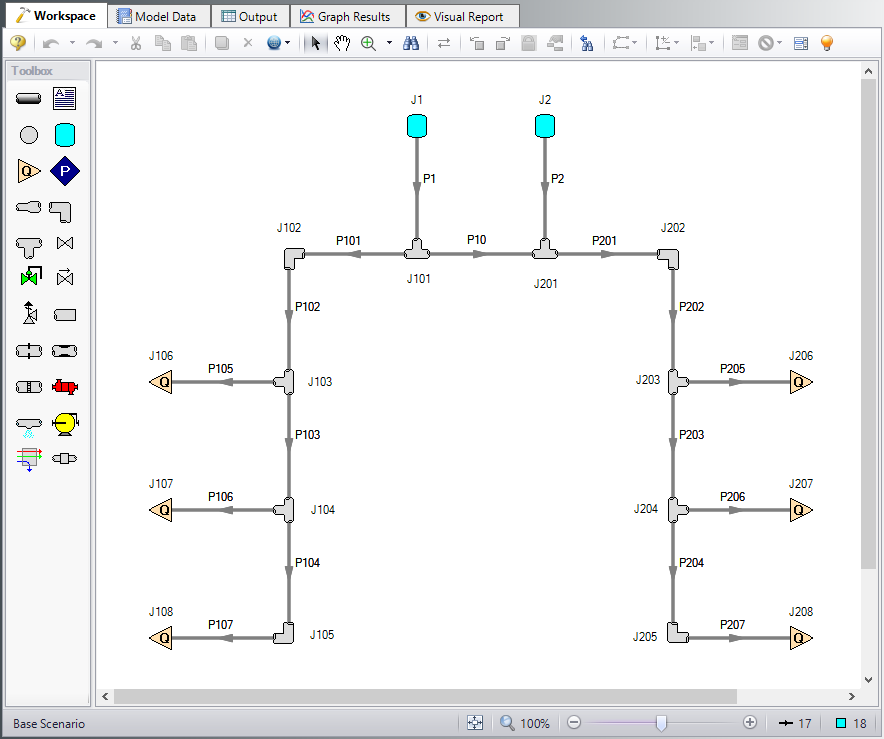
The system is in place but now we need to enter the properties of the objects. Double-click each pipe and junction and enter the following properties.
Pipe Properties
-
Pipe Model tab
-
Pipe Material = Steel - ANSI
-
Pipe Geometry = Cylindrical Pipe
-
Size = Use table below
-
Type = Use table below
-
Friction Model Data Set = Standard
-
Lengths = Use table below
-
| Pipe | Size (inch) | Type | Length (feet) |
|---|---|---|---|
| 1 | 12 | STD | 100 |
| 2 | 12 | STD | 150 |
| 10 | 12 | STD | 75 |
| 101 | 8 | STD (schedule 40) | 400 |
| 102-103 | 8 | STD (schedule 40) | 750 |
| 104 | 8 | STD (schedule 40) | 250 |
| 105 | 6 | STD (schedule 40) | 100 |
| 106 | 6 | STD (schedule 40) | 50 |
| 107 | 6 | STD (schedule 40) | 75 |
| 201 | 8 | STD (schedule 40) | 250 |
| 202-204 | 8 | STD (schedule 40) | 500 |
| 205 & 207 | 6 | STD (schedule 40) | 50 |
| 206 | 6 | STD (schedule 40) | 75 |
-
Heat Transfer tab
-
Heat Transfer Model = Convective Heat Transfer
-
Number of Insulation Layers = 1 External
-
Temperature = 75 deg. F
-
Fluid Velocity = 7 miles/hr
-
Insulation #1 Conductivity = 0.02 Btu/hr-ft-R
-
Insulation #1 Thickness = 2 inches
-
Junction Properties
-
-
J1 Name = Boiler 1
-
J2 Name = Boiler 2
-
Elevation = 0 feet
-
Pressure = 300 psia
-
Temperature = 800 deg. F
-
-
-
Elevation = 0 feet
-
Type = Smooth Bend (flanged or butt-welded)
-
Angle = 90 Degrees
-
r/D = 1.5
-
-
All Tee/Wye
-
Elevation = 0 feet
-
Loss Model = Detailed
-
Type = Tee (Sharp, straight run)
-
Initial Pressure = 100 psig (on Optional tab)
-
-
All Assigned Flows
-
Elevation = 0 feet
-
Type = Outflow
-
J106 Flow Rate = 40,000 lbm/hr
-
J107 Flow Rate = 50,000 lbm/hr
-
J108 Flow Rate = 60,000 lbm/hr
-
J206 Flow Rate = 55,000 lbm/hr
-
J207 Flow Rate = 40,000 lbm/hr
-
J208 Flow Rate = 60,000 lbm/hr
-
Note: Sometimes adding initial guesses to pipes or junctions can help difficult solutions converge.
ØTurn on Show Object Status from the View menu to verify if all data is entered. If so, the Pipes and Junctions group in Analysis Setup will have a check mark. If not, the uncompleted pipes or junctions will have their number shown in red. If this happens, go back to the uncompleted pipes or junctions and enter the missing data.
Step 4. Define the Steady Solution Control Group
There is an option available in Solution Control when using one of the marching methods that can sometimes result in an overall reduction in solution runtime. This option is to first solve the system using the Lumped Adiabatic method and then use these results as a starting point for the marching solution. Since the Lumped Adiabatic solution can typically be obtained much faster, this can provide an overall reduction in runtime for the marching method.
The Steady Solution Control Group is already defined using the default inputs. This means that no user input is required to run the model. However, the Lumped Adiabatic initialization will be used for this model.
To activate this option, do the following:
-
Open Analysis Setup
-
Navigate to the Solution Method panel in the Steady Solution Control group
-
Click the box to turn on First Use Lumped Adiabatic Method To Obtain Initial Stating Point For Marching Solution
The Steady Solution Control Group is now defined for this model.
Step 5. Run the Model
Click Run Model on the toolbar or from the Analysis menu. This will open the Solution Progress window. This window allows you to watch as the AFT Arrow solver converges on the answer. Once the solver has converged, view the results by clicking the Output button at the bottom of the Solution Progress window.
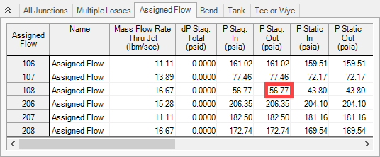
Step 6. Examine the Output
The pipes output section, shown in Figure 2, indicates the minimum delivery stagnation pressure is
Step 7. Solution Control Sensitivity
Open Analysis Setup and navigate to the Solution Method panel again. Change the Solution Method to User Specified with an Initial Number of Segments per Pipe as 10 (see Figure 3). Rerun the model, and compare the results to the previous run.
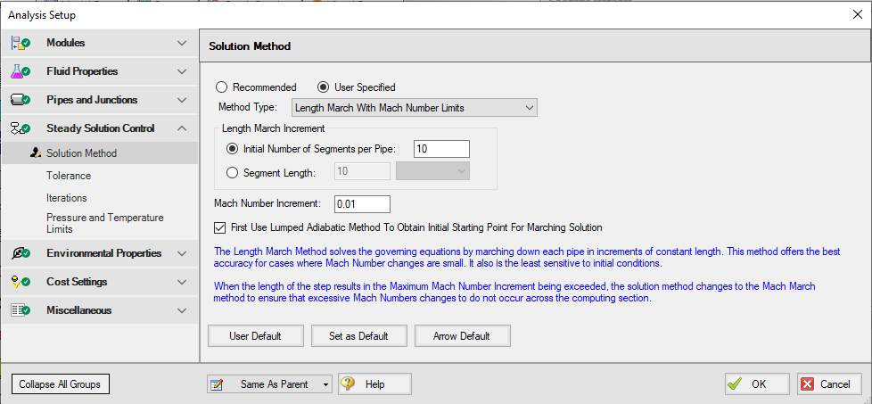
Repeat the run again with 20 segments, and 40 segments. What are the results?
-
With 2 segments, the minimum (stagnation) pressure is
-
With 10 segments, the minimum (stagnation) pressure is
-
With 20 segments, the minimum (stagnation) pressure is
-
With 40 segments, the minimum (stagnation) pressure is
This example points out the fact that some models are sensitive to the Solution Method used. While with most systems changing the solution control will not affect the results, in systems such as this were there are large pressure changes and high Mach numbers, the Solution Control settings can have a strong affect on the results. This is something that ALL engineers should be aware of, and keep in mind when creating computer model solutions.


