Refinery Relief System (English Units)
Refinery Relief System (Metric Units)
Summary
This example will demonstrate how to evaluate an emergency relief system for relief capacity, and mass and mole fraction of a discharge mixture for an environmental impact assessment.
Topics Covered
-
Evaluating Relief Valves
-
Using Scenarios
-
Using Global Junction Edit Feature
Required Knowledge
This example assumes the user has already worked through the Beginner: Air Heating System example, or has a level of knowledge consistent with that topic. You can also watch the AFT Arrow
Model File
This example uses the following file, which is installed in the Examples folder as part of the AFT Arrow installation:
Problem Statement
A new emergency relief system at an oil refinery is being considered, and the process calculations need to be evaluated.
The system provides relief to processes for methane, propane, and ethane. Each process is at
The relief valve CdA is
The process engineer has evaluated the relief capacity at the minimum process temperature of
Determine the following:
-
The relief capacity (i.e. flow rate) of each process.
-
The mass and mole fraction of the discharge mixture for the environmental impact assessment.
-
Determine if neglecting the high temperature case and the elevation effects are acceptable.
Step 1. Start AFT Arrow
From the Start Menu choose the AFT Arrow 9 folder and select AFT Arrow 9.
To ensure that your results are the same as those presented in this documentation, this example should be run using all default AFT Arrow settings, unless you are specifically instructed to do otherwise.
Step 2. Define the Steady Solution Control Group
There is an option available in Solution Control when using one of the marching methods that can sometimes result in an overall reduction in solution runtime. This option is to first solve the system using the Lumped Adiabatic method and then use these results as a starting point for the marching solution. Since the Lumped Adiabatic solution can typically be obtained much faster, this can provide an overall reduction in runtime for the marching method.
The Steady Solution Control Group is already defined using the default inputs. This means that no user input is required to run the model. However, the Lumped Adiabatic initialization will be used for this model.
To activate this option, do the following:
-
Open Analysis Setup
-
Navigate to the Solution Method panel in the Steady Solution Control group
-
Click the box to turn on First Use Lumped Adiabatic Method To Obtain Initial Stating Point For Marching Solution
The Steady Solution Control Group is now defined for this model.
Step 3. Define the Fluid Properties Group
-
Open Analysis Setup from the toolbar or from the Analysis menu
-
Open the Fluid panel then define the fluid:
-
Fluid Library = NIST REFPROP
-
Fluid = Methane
-
After selecting, click Add to Model
-
-
Repeat this to add Ethane and Propane
-
Specific Heat Ratio Source = Library
-
Step 4. Define the Pipes and Junctions Group
At this point, the first two groups are completed in Analysis Setup. The next undefined group is the Pipes and Junctions group. To define this group, the model needs to be assembled with all pipes and junctions fully defined. Click OK to save and exit Analysis Setup then assemble the model on the workspace as shown in the figure below.
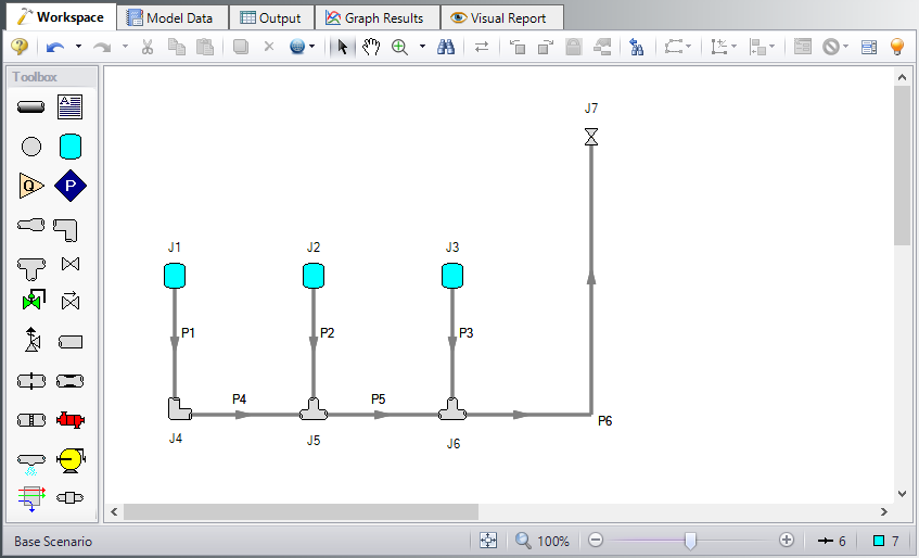
The system is in place but now we need to enter the properties of the objects. Double-click each pipe and junction and enter the following properties.
Pipe Properties
-
Pipe Model tab
-
Pipe Material = Steel - ANSI
-
Pipe Geometry = Cylindrical Pipe
-
Size = Use table below
-
Type = STD (schedule 40)
-
Friction Model Data Set = Standard
-
Lengths = Use table below
-
| Pipe | Size (inch) | Length (feet) |
|---|---|---|
| 1-3 | 3 | 50 |
| 4 | 3 | 25 |
| 5 | 4 | 25 |
| 6 | 6 | 150 |
Junction Properties
-
All Tanks
-
J1 Name = Methane Tank
-
J2 Name = Ethane Tank
-
J3 Name = Propane Tank
-
Elevation = 0 feet
-
J1 Fluid = Methane
-
J2 Fluid = Ethane
-
J3 Fluid = Propane
-
Pressure = 200 psig
-
Temperature = 300 deg. F
-
-
J4 Bend
-
Elevation = 0 feet
-
Type = Standard Elbow (knee, threaded)
-
Angle = 90 Degrees
-
-
All Tees
-
Elevation = 0 feet
-
Loss Model = Simple
-
-
J7 Valve
-
Name = Relief Valve
-
Elevation = 0 feet
-
Valve Data Source = User Specified
-
Subsonic Loss Model = K Factor
-
K = 0
-
CdA (for Sonic Choking - optional) = 15 inches2
-
Exit Valve (optional) = Checked
-
Exit Pressure = 0 psig
-
Exit Temperature = 70 deg. F
-
ØTurn on Show Object Status from the View menu to verify if all data is entered. If so, the Pipes and Junctions group in Analysis Setup will have a check mark. If not, the uncompleted pipes or junctions will have their number shown in red. If this happens, go back to the uncompleted pipes or junctions and enter the missing data.
Step 5. Run the Model
Click Run Model on the toolbar or from the Analysis menu. This will open the Solution Progress window. This window allows you to watch as the AFT Arrow solver converges on the answer. Once the solver has converged, view the results by clicking the Output button at the bottom of the Solution Progress window.
Step 6. Specify the Output Control
Open the Output Control window by selecting Output Control from the Toolbar or Tools menu.
With the Pipes button selected at the top, add Concentration Mass Fraction and Concentration Mole Fraction to the pipe output list by highlighting these parameters (holding CTRL will allow you to select both at the same time) and then clicking the purple Add arrow.
Step 7. Examine the Output
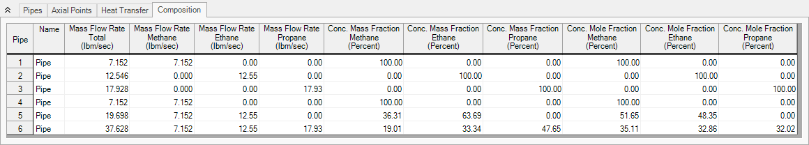
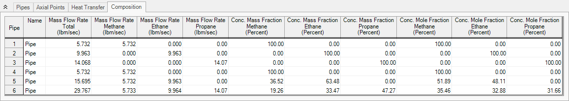
The Composition tab in the pipes output section displays the component mass flow rate through each of the pipes, as shown in Figure 2).
The output for this model shows:
-
The total relief capacity is 37.628 lbm/sec
-
7.152 lbm/sec for methane
-
12.55 lbm/sec for ethane
-
17.93 lbm/sec for propane
-
-
The mass fraction at discharge (observed from clicking on the Composition tab): 19.01% methane, 33.34% ethane, and 47.65% propane
-
The mole fraction at discharge from the Composition tab: 35.11% methane, 32.86% ethane, and 32.02% propane
Step 8. Create a Child Scenario
In order to determine if the process engineer has made good assumptions by neglecting the higher temperature process and the elevation data, it will be necessary to change the model. This can be done easily using the Scenario Manager on the Quick Access Panel. Note that the Scenario Manager can also be accessed from the Tools menu.
The Scenario Manager is a powerful tool for managing variations of a model, referred to as scenarios.
The Scenario Manager allows you to:
-
Create, name and organize scenarios
-
Select the scenario to appear in the Workspace (the ‘current’ scenario)
-
Delete, copy and rename scenarios
-
Duplicate scenarios and save them as separate models
-
Review the source of a scenario’s specifications
-
Pass changes from a scenario to its variants
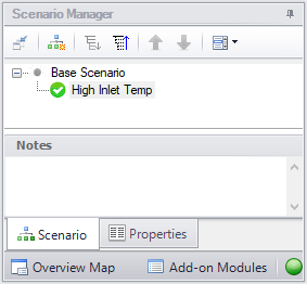
The Scenario Manager should currently appear as shown in Figure 3.
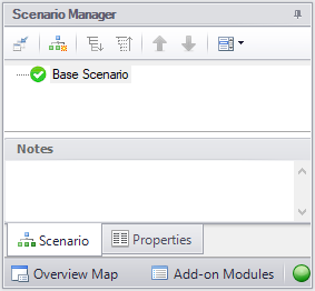
Figure 3: The Scenario Manager window on the Quick Access Panel is used to create and manage model scenarios
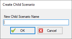
Create a child scenario by either right-clicking on the Base Scenario and then selecting Create Child. Enter the name High Inlet Temp in the Create Child Scenario window, as shown if Figure 4. Click OK. The new High Inlet Temp scenario should now appear in the Scenario Manager on the Quick Access Panel below the Base Scenario as shown in Figure 5.
Step 9. Modify the Higher Inlet Temp Scenario with Global Junction Editing
Double-click on the High Inlet Temp scenario in the Scenario Manager on the Quick Access Panel to make it the active scenario if it is not already.
To check the process engineer's assumption about the
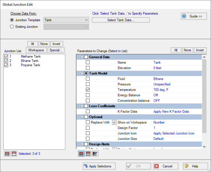
AFT Arrow has a feature that can be used to change the temperature for all of the tanks at the same time. This feature is called Global Junction Editing.
Open the Global Junction Edit window by selecting Global Junction Edit | Tanks from the Edit menu. Select all of the tanks in the Junction List by clicking All at the top (see Figure 6).
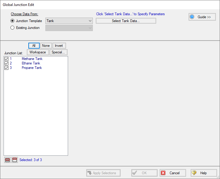
Click the Select Tank Data button. This will open a Tank Properties window. Enter a temperature of
Step 10. Run the Model
Click Run Model on the toolbar or from the Analysis menu. This will open the Solution Progress window. This window allows you to watch as the AFT Arrow solver converges on the answer. Once the solver has converged, view the results by clicking the Output button at the bottom of the Solution Progress window.
Step 11. Examine the Output
See Figure 8 for the output from this scenario. The output for this model shows:
At
Step 12. Create and Run a Child Scenario for Elevation Effects
Create a child scenario to the High Inlet Temp scenario to examine the affect including the elevation information has on the model.
Change the elevation data for the J7 Valve to
Adding the


