Air Receiver Tank - XTS
(English Units)
Air Receiver Tank - XTS (Metric Units)
Summary
The objective of this example is to introduce the user to the Extended Time Simulation (XTS) module by modeling the pressurizing of an air receiver tank. A positive displacement compressor is used to charge the tank and is shut off once the required pressure is reached for a compressed air process.
Note: This example can only be run if you have a license for the XTS module.
Topics Covered
-
Specifying the Transient Control group
-
Understanding Transient Output
Required Knowledge
This example assumes the user has already worked through the Beginner: Air Heating System example, or has a level of knowledge consistent with that topic. You can also watch the AFT Arrow
Model File
This example uses the following file, which is installed in the Examples folder as part of the AFT Arrow installation:
Step 1. Start AFT Arrow
From the Start Menu choose the AFT Arrow 9 folder and select AFT Arrow 9.
To ensure that your results are the same as those presented in this documentation, this example should be run using all default AFT Arrow settings, unless you are specifically instructed to do otherwise.
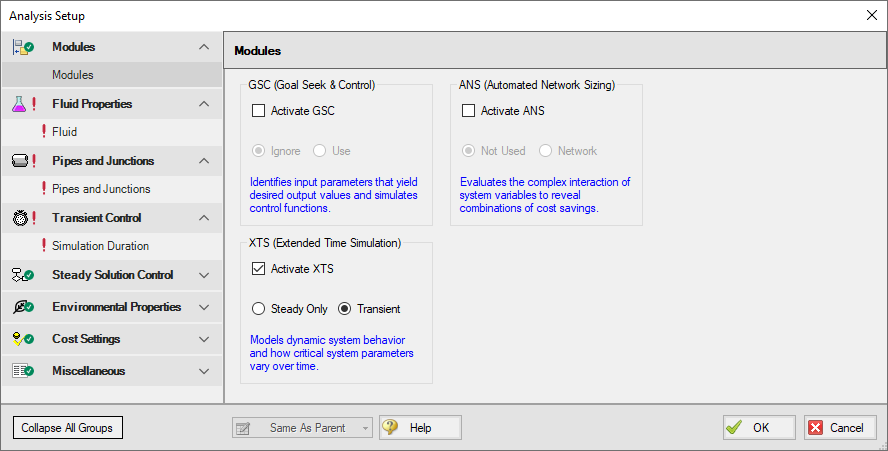
Step 2. Define the Modules Panel
Open Analysis Setup from the toolbar or from the Analysis menu. Navigate to the Modules panel. For this example, check the box next to Activate XTS and select Transient to enable the XTS module for use. Note that XTS can also be enabled from the Analysis menu by going to the Time Simulation option and selecting Transient, as shown in Figure 1. When XTS is activated a new group will appear in Analysis Setup titled Transient Control.
Step 3. Define the Fluid Properties Group
-
Open Analysis Setup from the toolbar or from the Analysis menu
-
Open the Fluid panel then define the fluid:
-
Fluid Library = AFT Standard
-
Fluid = Air
-
After selecting, click Add to Model
-
-
Equation of State = Redlich-Kwong
-
Enthalpy Model = Generalized
-
Specific Heat Ratio Source = Library
-
Step 4. Define the Pipes and Junctions Group
At this point, the first two groups are completed in Analysis Setup. The next undefined group is the Pipes and Junctions group. To define this group, the model needs to be assembled with all pipes and junctions fully defined. Click OK to save and exit Analysis Setup then assemble the model on the workspace as shown in the figure below.
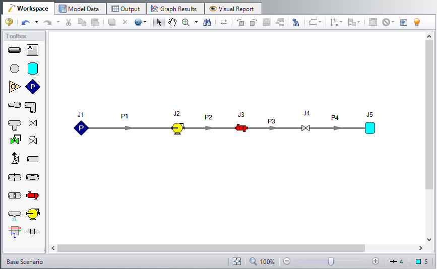
The system is in place but now we need to enter the properties of the objects. Double-click each pipe and junction and enter the following properties.
Pipe Properties
-
Pipe P1
-
Pipe Material = Steel - ANSI
-
Pipe Geometry = Cylindrical Pipe
-
Size = 3 inch
-
Type = STD (schedule 40)
-
Friction Model = Standard
-
Length =
-
-
Pipes P2 - P4
-
Pipe Material = Steel - ANSI
-
Pipe Geometry = Cylindrical Pipe
-
Size = 3 inch
-
Type = STD (schedule 40)
-
Friction Model = Standard
-
Length =
-
Junction Properties
-
J1 Assigned Pressure
-
Elevation = 0
-
Fluid = Air
-
Stagnation Pressure = 0
-
Stagnation Temperature =
-
-
J2 Compressor
-
Elevation = 0
-
Compressor Model = Positive Displacement Compressor
-
Compression Process Thermodynamics = Polytropic
-
Polytropic Constant = 1.2
-
Compressor Sizing Parameter = Mass Flow Rate
-
Fixed Flow Rate =
-
Note: The polytropic constant entered for the compressor is intended to represent an active cooling element in the compressor.
-
J3 Heat Exchanger
-
Elevation = 0
-
On the Loss Model Data tab
-
Select the Loss Model as Resistance Curve, and then click the Enter Curve Data button
-
Select the Flow Parameter as Mass with units of
-
Enter
-
Click Fill as Quadratic to create data for a square loss curve
-
Click Generate Curve Fit Now to create a quadratic curve fit
-
-
On the Thermal Data tab:
-
Thermal Model = Controlled Downstream Temperature
-
Controlled Outlet Temperature =
-
-
-
J4 Valve
-
Elevation = 0
-
Loss Model = User Specified
-
Subsonic Loss Model = Cv (ANSI/ISA)
-
Loss Source = Fixed Cv
-
Cv = 50
-
Xt = 0.7
-
-
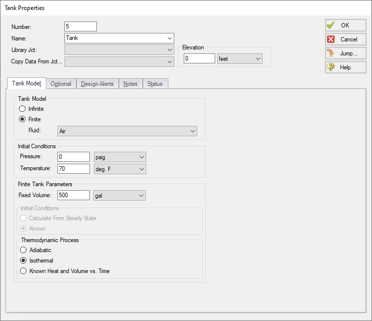
J5 Tank
-
Tank Model = Finite
-
Initial Conditions
-
Pressure = 0
-
Temperature =
-
-
Finite Tank Conditions
-
Fixed Volume =
-
Initial Conditions = Known
-
Thermodynamic Process = Isothermal
-
-
ØTurn on Show Object Status from the View menu to verify if all data is entered. If so, the Pipes and Junctions group in Analysis Setup will have a check mark. If not, the uncompleted pipes or junctions will have their number shown in red. If this happens, go back to the uncompleted pipes or junctions and enter the missing data.
Step 5. Define the Transient Control Group
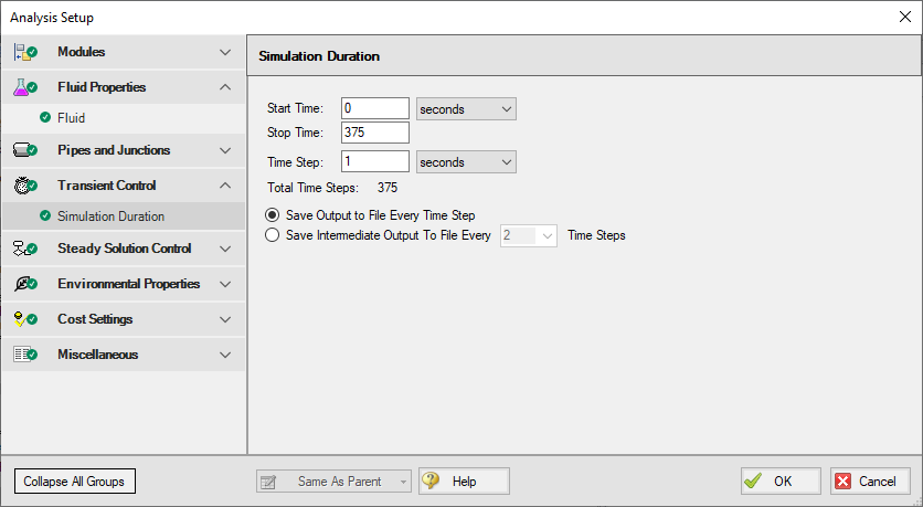
XTS module transient simulations are controlled through the Simulation Duration panel. You can access the Simulation Duration panel by selecting Transient Control from the Analysis Menu, navigating to the Simulation Duration item in Analysis Setup, or by clicking the Simulation Duration shortcut on the Common Toolbar. When the time simulation mode is set to Steady-Only AFT Arrow will ignore the input in the Simulation Duration panel. When AFT Arrow is set to perform a transient analysis, the Transient Control group becomes a required item before the model can run. Use the Simulation Duration panel to specify transient start and stop times, set time steps, specify the number of output points that are saved to the transient output file (allows XTS to do transient calculations with a small time step while limiting the size of the transient data output file), and adjust solution parameters for finite tank liquid level calculations. Specify start times, stop times, and time steps in any units from seconds to years.
Set the Start Time to 0 seconds and the Stop Time as 375 seconds, with a time step of 1 second. The output will be saved to the output file for every time step. The Simulation Duration panel should appear as shown in Figure 4.
Step 6. Set Up the Compressor Transient
In the XTS module, you can define transients for junctions. These transients include events such as valves opening and closing and compressors starting and shutting down. Transients for junctions are defined as either time-based or event-based transients. A time-based transient starts at a specified absolute time. Event based transients initiate when a defined criteria, such as a specified pressure in a particular pipe is reached. There are three types of event transients for junctions: single event, dual event cyclic, and dual event sequential. Single event transients are events that occur only once in a simulation. Dual cyclic events are two transient events that repeat one after the other as many times as the event trigger occur during a simulation (such as a valve closing then reopening). Dual sequential transient events are two transient events which occur one after the other, without repeating.
For this example, set a single event-based transient on the compressor so the compressor will shut off over 30 seconds when the pressure at the tank inlet reaches
Open the Compressor Properties window for compressor J2 and navigate to the Transient tab. Under Initiation of Transient, select Single Event and enter the Transient data as shown below in Figure 5.
Step 7. Run the Model
After defining all of the pipes and junctions transient data and transient control items, the transient model can run. Click Run Model from the Common Toolbar or Analysis menu.
When using the XTS module, the Solution Progress window displays the progress through the transient analysis. This information is displayed below the solution tolerance data, as shown in Figure 6.
After the run finishes, view the results by clicking the Output button.
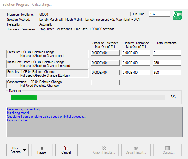
Figure 6: Solution Progress Window shows the convergence progress, as well as the transient solution progress when running transient cases
Step 8. Examine the Transient Results
AFT Arrow displays transient output for all Pipes and Junctions in the Output Window, as shown in Figure 7.
![]()
Figure 7: Transient output is displayed in the Output Window
Each of the summary tables in the General Output section has a companion transient summary tab which displays the summary data at each time step in the transient run. Each junction included in the summary is included in the transient summary. The transient summary data for each junction may be expanded or collapsed by clicking the + or – sign in beside the junction data list. The entire list may be expanded or collapsed by clicking the button in the top left-hand corner of the transient summary window. Figure 8 shows the Tank Transient summary tab, with all of the data sets collapsed. Figure 9 shows the Tank Transient summary tab, with the data for the J5 Tank expanded.
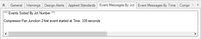
The Event Messages tabs in the General Section (Figure 10) can be used to see when events are triggered during the transient. For this example the Event Messages By Jct tab shows that the flow transient at the compressor was triggered at
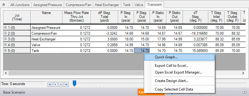
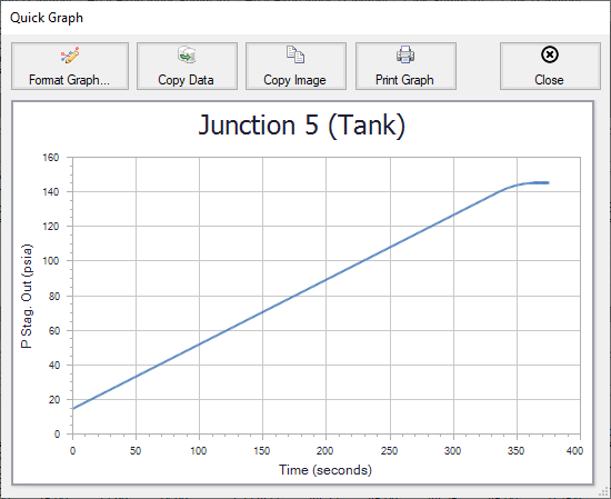
The Quick Graph feature can be used to plot transient data for rapid examination. To use the Quick Graph feature, place the mouse cursor over the column of data you wish to examine. Then, right click with the mouse, and select Quick Graph from the list. Figure 11 illustrates how to generate a Quick Graph for J5 Tank Pressure vs. Time. The graph illustrates how the pressure in the tank rises over time and steadies out at about
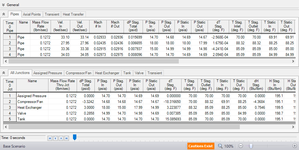
Similar to the summary transient data, the transient tabs in the Pipe and Junctions sections of the Output Window (shown in Figure 7) are used to display the transient data for each pipe and junction at every time step. This transient data can be expanded or collapsed in the same manner as in the General Output transient summaries.
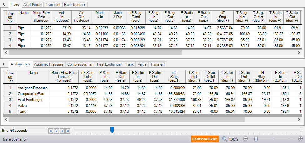
Figure 13 shows the output data for the pipes and junctions, found on the Pipes and All Junctions tabs, at the initial time step, Time = 0 seconds. The output for all of the pipes and junctions can be displayed at any time step by using the slider bar located at the bottom of the Output window. Figure 14 shows the pipe and junction data at Time = 60 seconds.