When Goals Cannot Be Achieved
In some cases the GSC module may not be able to achieve a goal. This can happen for the following reasons:
-
A goal is not physically realistic
-
A better starting point is needed for the input values assigned as GSC Variables
-
Hydraulic solution tolerances or optimizer numerical parameters require adjustment
In such cases, the goal will not be satisfied in the results. In other words, the Actual Goal Value and User Goal Value will differ (Figure 1).
In all cases the user will be warned when goals were not met. Figure 1 shows the Output window with such a warning.
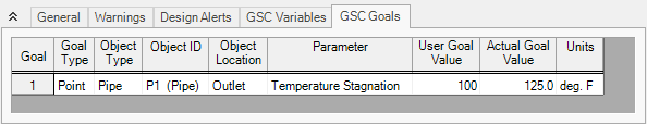
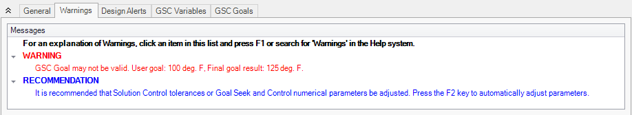
Figure 1: Warning display in Output window when a goal cannot be met
Physically unrealistic goals
It may be possible that a goal is not achievable because it is not physically possible. For example, a compressor/fan may be too small to satisfy a flowrate goal at some pipe.
To determine whether a goal is unrealistic, try changing the goal and rerunning the model. If the goal can be met in some cases and not others, this is an indicator that the original goal was unrealistic.
Better starting point needed
In some cases the goal may be so far away from the original model that the GSC module has difficulty finding a solution. This is not common, but it is worth trying to adjust the starting point of parameters which are being varied.
Changing control parameters
The Numerical Optimizer determines goal search directions by approximating a gradient based on perturbed variable values. By default it uses a central difference approximation, but forward difference can also be used. If the hydraulic solution is not converged to a sufficiently small tolerance, the gradient approximation will not be sufficiently accurate and hence a good search direction cannot be obtained. The end result is that the goal seeking fails.
There are two general areas that can be changed in such cases: the hydraulic solution tolerances in the Tolerance panel, and numerical control parameters in the Numerical Controls panel.
In the next few sections recommendations on how to manually change these parameters will be given. However, before making a manual change it is definitely worth trying the automated parameter adjustment feature.
Figure 1, bottom picture, shows the warning when a goal is not met, and also shows a recommendation and suggests pressing the “F2” key. When doing so, a window appears as shown in Figure 2. This window will offer up to three options for automatic parameter adjustment. It is typically a good idea to accept the default changes, click OK, and rerun the model.
The purpose of the Figure 2 window is to simplify for the user making common changes to resolve goal seeking problems.
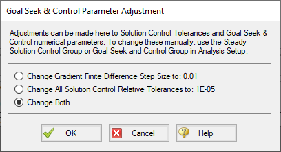
Figure 2: When goal seeking fails, pressing the F2 key will show this window which allows the user to automatically implement recommend numerical parameter adjustments
Caution: The user should be very cautious in manually changing parameters in the Tolerance panel and the Numerical Controls panel. Making changes without a good understanding of the parameters involved can lead to incorrect results.
-
Changing tolerance in Steady Solution Control Group >Tolerance panel- By default AFT Arrow uses Relative Tolerance criteria set to 0.0001 (see Figure 3). Goal seeking convergence can sometimes be improved by reducing these values to 0.00001 or 0.000001.
See Tolerance panel for a more in-depth discussion.
-
Changing goal seeking numerical control - Figure 4 shows the Numerical Controls panel in Analysis Setup. The most useful parameter one can adjust is the Relative Finite Difference Step Size. Using values between 0.01 and 0.001 are recommended. In some cases using a value as high as 0.1 may be tried.
-
Changing Multi-Variable Goal Weighting - When two or more variables (and, hence two or more goals) are applied, the relative influence of each goal is important. By default, the GSC module "normalizes" each goal. This means that the difference between each goal and the current value is divided through by the goal. A Root Mean Square (RMS) of all normalized values is then taken, and this function is then driven to zero. The normalization approach tends to work better in cases where the numerical values of different goals are very different.
There are two other options available. These can be selected on the Numerical Controls panel (Figure 4). The second option is to not normalize the goals. Each goal is then subtracted from the current value, and an RMS is taken of the differences. This becomes the function that is driven to zero. This method tends to work best when the numerical values of the goals are similar in magnitude.
A final option is for the user to input weighting factors. This approach uses the normalized approach described previously, but multiplies each normalized value by a user specified weighting factor before performing the RMS. The general approach here is if one or more of the goals is not being reached, increase its weighting factor. The weighting factors are entered into a column in the goals table on the Goals panel. This column will become visible when the third option is chosen.
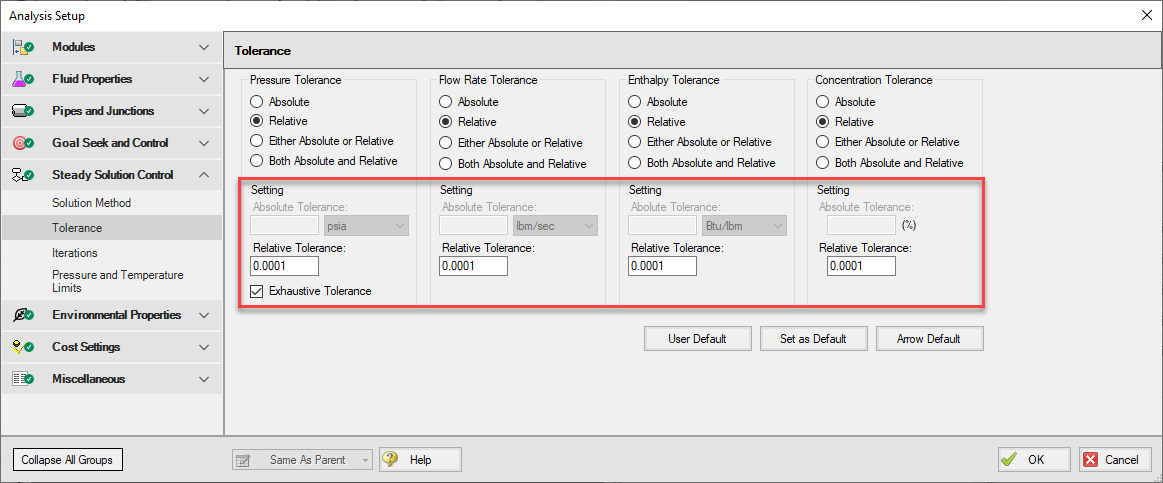
Figure 3: Reducing tolerance criteria may resolve goal seeking difficulties
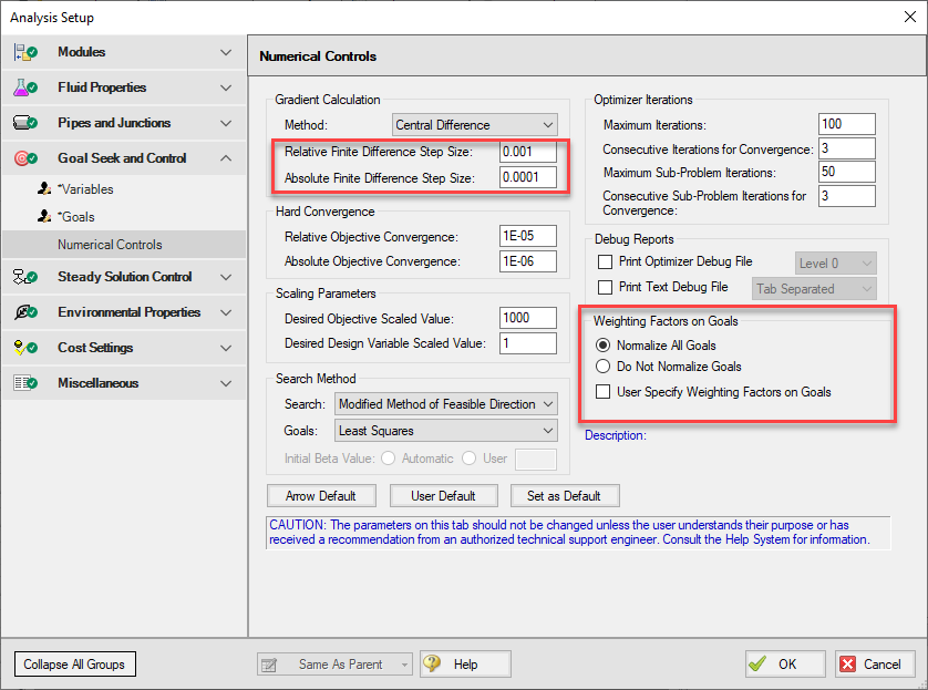
Figure 4: Changing certain numerical control parameters in the Numerical Controls panel may resolve goal seeking difficulties


