Centrifugal Compressor
Analysis Type
This topic pertains to the Centrifugal Compressor Curve Analysis option which represents the real behavior of a centrifugal compressor or fan. For Sizing Analyses, see Compressor/Fan Sizing.
Centrifugal Compressor Curve
A single compressor curve is useful if the compressor will operate at a fixed speed. The right side of the Compressor Model tab displays the defined curve(s) for the compressor.
To enter curves, click Enter Curve Data. Once this data has been defined, previews of the applied curves can be seen on the right side of the Compressor Model tab. Note that only one curve can be entered unless different configurations under the Multiple Configurations tab have been specified.
A Compressor Map is a family of compressor curves categorized by different operating speeds and is typically provided by a manufacturer in the form of a graph or data sheet. These curves can be input into AFT Arrow which uses an extension of the Multiple Configurations feature. The Solver will use the Rated Speed entered by the user to interpolate between the available curves and determine the actual operating point.
When to Use a Compressor Map
-
The working fluid of the AFT Arrow model is the same as the fluid used by the manufacturer when developing the Compressor Map.
-
Manufacturer data is provided in units of non-dimensional or corrected mass flowrate vs pressure ratio.
-
The AFT Arrow model needs to account for inlet temperatures and pressures that differ from the manufacturer test conditions.
-
Various scenarios that use different operating conditions or speeds need to be analyzed. The Compressor Map will characterize a range of operating conditions rather than being constrained to a single curve.
Entering or Modifying Compressor Map Curves
-
Select the Compressor Map radio button under the Centrifugal Compressor model.
-
Click Enter Curve Data under the Compressor Curve area which will open the Compressor Map window.
-
Select the appropriate flow parameter and units in the Raw Data table header rows (Non-dimensional or Corrected Mass Flow).
-
Enter the data for one of the curves into the table.
-
Specify the Curve Fit type (Polynomial or Interpolated X-Y Data) and click Graph Data Now / Generate Curve Fit Now.
-
Specify the Reference Inlet Conditions which are the pressure and temperature of the fluid used by the manufacturer when generating the Compressor Map curves.
-
Enter a Non-dimensional or Corrected Speed associated with the curve under the Configuration Information area on the right side of the Compressor Map window. An optional description can also be entered.
-
Click Update Configuration Now which will add the curve and associated speed to the list at the top-right of the Compressor Map window.
-
Click Create and repeat the above steps to enter the next curve for a different speed. Repeat this process until all desired curves are entered and categorized in the list.
-
Once all the curves are entered, click OK to accept and close the Compressor Map window.
-
Enter a Rated Speed on the Compressor/Fan Properties window. The Solver will use this speed to interpolate between the available curves.
Compressor Maps can be modified by clicking Enter Curve Data, selecting the speed from the list in the top-right, modifying the data of interest, clicking Graph Data Now / Generate Curve Fit Now, and clicking Update Configuration Now.
Viewing Compressor Map Curves - Individual curves can be viewed by changing the Speed dropdown menu on the Compressor/Fan Properties window, or by using the Composite Graph, Performance Graph, or Efficiency Graph tabs on the Compressor Map window.
Surge and Stall Lines - The Surge Line is described by connecting the data points with the lowest flowrate for each speed curve. The Stall Line is described by connecting the data points with the highest flowrate for each speed curve. These two lines bound the preferred range of operation inside the Compressor Map, and a Warning will be given if the corrected or non-dimensional flow is outside this range. Furthermore, a Warning will be given if the corrected or non-dimensional speed is outside the range of the data.
Variable Speed tab - The Fixed Speed (%) field will directly scale the Rated Speed that was entered on the Compressor/Fan Properties window. Note that the Affinity Laws are NOT used unlike the normal compressor curve.
Output - Corrected Mass Flow, Stagnation Pressure Ratio, and other useful output parameters are available within the Output Control.
Added Pressure
If the compressor curve is entered using pressure rise information as opposed to a head rise, the pressure rise will need to be specified as either a stagnation or static pressure. This specification is performed on the Compressor Model tab under the Centrifugal compressor specification. Note that mechanical energy rises are typically entered in Arrow as pressure rises instead of head rises because the usefulness of the head term in variable-density systems is diminished.
Compression Process Thermodynamics
Depending on the compression process, significant thermal effects can occur. Fans and blowers create a pressure rise that is typically so low that the temperature is not noticeably affected, which is why Arrow treats the Fan model as adiabatic, but the large pressure rise in compressors leads to significant temperature changes. This is also known as the heat of compression, and in Arrow it can be accounted for in a compressor in multiple ways:
-
Isentropic - The compressor is treated as 100% efficient using an isentropic efficiency. If the compression process is isentropic, the temperature rise is given by the following relationship:

where the pressures and temperatures are static and not stagnation. Gamma (γ) is the specific heat ratio.
-
Polytropic - If there is incidental heat loss to ambient, or if the compressor is actively cooled, the process will not be adiabatic. In this case the process is referred to as polytropic, and the temperature rise is given by the following:

where n is the polytropic exponent. If n is equal to γ, it is isentropic. Typically, n is greater than γ for compressors.
-
Determine From Efficiency Data - If efficiency data is entered as optional data in the Compressor curve, this option can be selected and the thermal effects of the compressor due to compression heating will be calculated. The efficiency data will be applied as isentropic efficiency, which is defined as the ideal work for an isentropic process over the actual work.
Check Valve at Discharge (No Backflow Allowed)
If this option is checked when modeling a centrifugal compressor with a compressor curve, a check valve that can be considered part of the compressor itself is assumed to exist. This will never allow backflow at the compressor junction. If a check valve closes as part of the steady-state simulation, Arrow will perform recalculations under the assumption that the compressor's check valve is closed. Note that a steady check valve position must be attained in order for Arrow to apply its steady-state calculations.
-
Forward Velocity to Close - The flow velocity, in the forward direction, that causes the check valve to close, preventing any further flow. A negative value in this field indicates that a reverse flow below the specified value will be permitted through the compressor before it closes.
-
Delta Head to Re-Open - The differential head or pressure (upstream minus downstream) required to re-open the check valve.
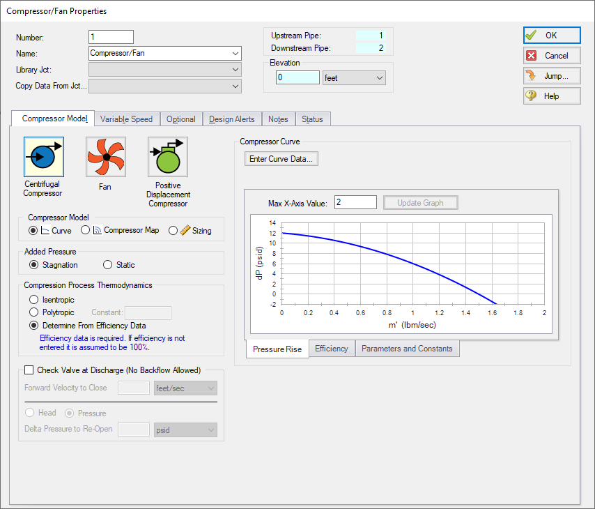
Figure 1: Compressor model with a centrifugal compressor curve defined


