Compressed Air System

Compressed Air System - GSC (Metric Units)

Compressed Air System - GSC (English Units)

Summary

The objective of this example is to demonstrate how multiple goals and variables are used in the GSC module to achieve an objective.

Note: This example can only be run if you have a license for the GSC module.

Topics Covered

Defining the Goal Seek and Control group
Setting Variables and Goals
Applying multiple Variables and Goals
Interpreting Goal Seek and Control Output

Required Knowledge

This example assumes the user has already worked through the Beginner: Air Heating System example, or has a level of knowledge consistent with that topic. You can also watch the AFT Arrow Quick Start Video (Metric Units) on the AFT website, as it covers the majority of the topics discussed in the Beginner: Air Heating System example.

In addition the user should have worked through the Beginner: Heat Transfer in a Pipe - GSC example.

Model Files

This example uses the following files, which are installed in the Examples folder as part of the AFT Arrow installation:

Problem Statement

For this example, we will use the GSC module to determine the valve K-factors required to achieve a specified flow of 55 gram/sec to all four tools.

Step 1. Start AFT Arrow

From the Start Menu choose the AFT Arrow 9 folder and select AFT Arrow 9.

To ensure that your results are the same as those presented in this documentation, this example should be run using all default AFT Arrow settings, unless you are specifically instructed to do otherwise.

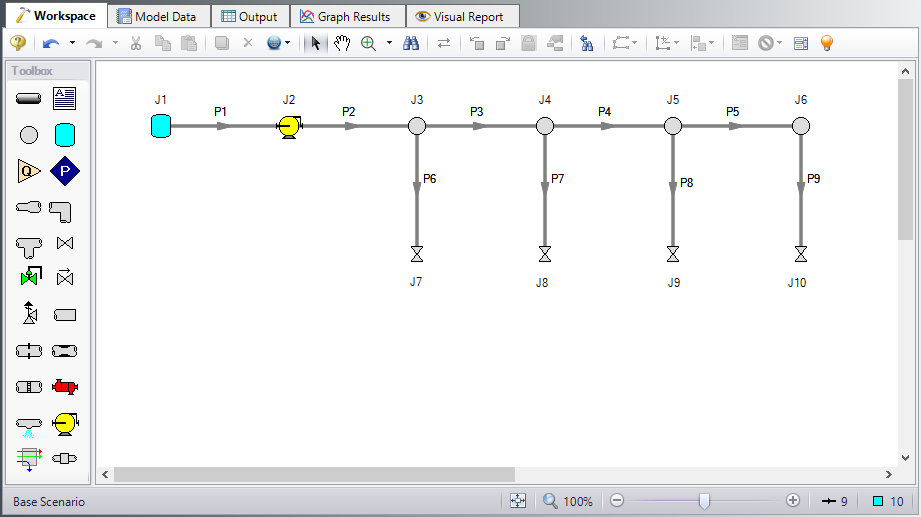
Open the Metric - Compressed Air System.aro example file listed above, which is located in the Examples folder in the AFT Arrow application folder. Save the file to a different folder. This is the only scenario needed for this example, so right-click the Base Scenario and select Delete All Children. The workspace should look like Figure 1.

Figure 1: Model Layout for GSC Compressed Air System Example

Step 2. Define the Steady Solution Control Group

There is an option available in Solution Control when using one of the marching methods that can sometimes result in an overall reduction in solution runtime. This option is to first solve the system using the Lumped Adiabatic method and then use these results as a starting point for the marching solution. Since the Lumped Adiabatic solution can typically be obtained much faster, this can provide an overall reduction in runtime for the marching method.

The Steady Solution Control Group is already defined using the default inputs. This means that no user input is required to run the model. However, the Lumped Adiabatic initialization will be used for this model.

To activate this option, do the following:

Open Analysis Setup
Navigate to the Solution Method panel in the Steady Solution Control group
Click the box to turn on First Use Lumped Adiabatic Method To Obtain Initial Stating Point For Marching Solution

The Steady Solution Control Group is now defined for this model.

Step 3. Define the Pipes and Junctions Group

Make the following changes to these junctions:

J7-J10 Valves
1. Subsonic Loss Model = K Factor
2. K = 10

Step 4. Define the Modules Group

Navigate to the Modules panel in Analysis Setup. Check the box next to Activate GSC. The Use option should automatically be selected, making GSC enabled for use.

Step 5. Define the Goal Seek and Control Group

Specify the variables and goals for the model using the Goal Seek and Control group in Analysis Setup.

Variables Panel

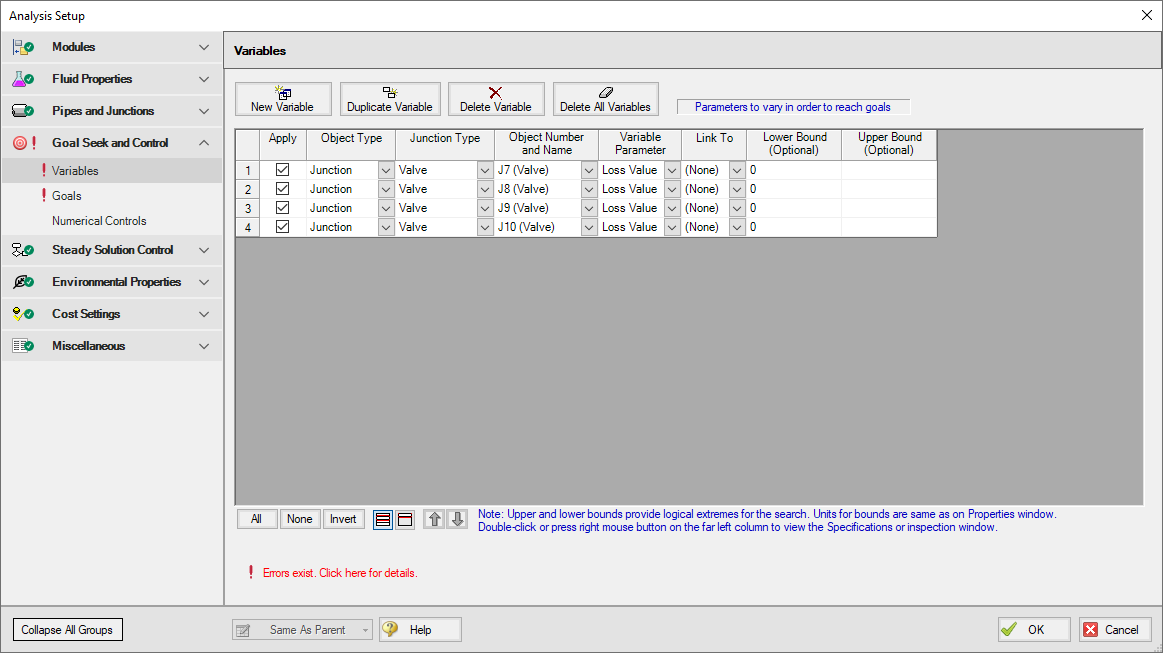
Open the Variables panel, click New Variable, and enter the following variable data:

J7 Valve
1. Apply = Selected
2. Object Type = Junction
3. Junction Type = Valve
4. Junction Number and Name = J7 (Valve)
5. Variable Parameter = Loss Value
6. Link To = (None)
7. Lower Bound = 0
8. Upper Bound = Leave blank
J8 Valve
1. Apply = Selected
2. Object Type = Junction
3. Junction Type = Valve
4. Junction Number and Name = J8 (Valve)
5. Variable Parameter = Loss Value
6. Link To = (None)
7. Lower Bound = 0
8. Upper Bound = Leave blank
J9 Valve
1. Apply = Selected
2. Object Type = Junction
3. Junction Type = Valve
4. Junction Number and Name = J9 (Valve)
5. Variable Parameter = Loss Value
6. Link To = (None)
7. Lower Bound = 0
8. Upper Bound = Leave blank
J10 Valve
1. Apply = Selected
2. Object Type = Junction
3. Junction Type = Valve
4. Junction Number and Name = J10 (Valve)
5. Variable Parameter = Loss Value
6. Link To = (None)
7. Lower Bound = 0
8. Upper Bound = Leave blank

After entering the data, the Variables tab should appear as shown in Figure 2.

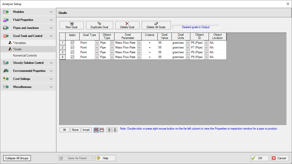
Figure 2: Goal Seek and Control group, Variables panel is used to specify the variables

Goals Panel

Open the Goals panel, click New Goal, and enter the following goal data:

Pipe P6
1. Apply = Selected
2. Goal Type = Point
3. Object Type = Pipe
4. Goal Parameter = Mass Flow Rate
5. Criteria = =
6. Goal Value = 55
7. Goal Units = gram/sec
8. Object ID = P6 (Pipe)
9. Object Location = NA
Pipe P7
1. Apply = Selected
2. Goal Type = Point
3. Object Type = Pipe
4. Goal Parameter = Mass Flow Rate
5. Criteria = =
6. Goal Value = 55
7. Goal Units = gram/sec
8. Object ID = P7 (Pipe)
9. Object Location = NA
Pipe P8
1. Apply = Selected
2. Goal Type = Point
3. Object Type = Pipe
4. Goal Parameter = Mass Flow Rate
5. Criteria = =
6. Goal Value = 55
7. Goal Units = gram/sec
8. Object ID = P8 (Pipe)
9. Object Location = NA
Pipe P9
1. Apply = Selected
2. Goal Type = Point
3. Object Type = Pipe
4. Goal Parameter = Mass Flow Rate
5. Criteria = =
6. Goal Value = 55
7. Goal Units = gram/sec
8. Object ID = P9 (Pipe)
9. Object Location = NA

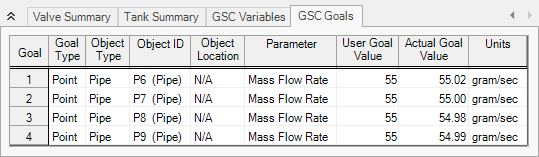
After entering the data, the Goals tab should appear as shown in Figure 3.

Figure 3: Use the Goals panel is used to specify the goals

Step 6. Run the Model

Click Run Model on the toolbar or from the Analysis menu. This will open the Solution Progress window. This window allows you to watch as the AFT Arrow solver converges on the answer. Once the solver has converged, view the results by clicking the Output button at the bottom of the Solution Progress window.

Step 7. Examine the Output

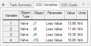
The results of the GSC analysis are shown in the General Output section. The GSC Variables tab shows the final value for the variable parameter, as shown in Figure 4. The GSC Goals tab shows the final value achieved for the goal, as shown in Figure 5.

The GSC module analysis determined the following valve K-factors would result in the desired flow of 55 gram/sec to each valve:

Object	Value
J7	13.98
J8	11.48
J9	10.38
J10	10.08

Figure 4: GSC Variable Results are displayed in the General section of the Output window

Figure 5: GSC Goal Results are displayed in the General section of the Output window