Steam Relief System - GSC (English Units)

Summary

The objective of this example is to demonstrate how goals and variables are used in the GSC module to achieve an objective.

Note: This example can only be run if you have a license for the GSC module.

Topics Covered

• Defining the Goal Seek and Control group

• Setting Variables and Goals

• Understanding Goal Seek and Control output

Required Knowledge

This example assumes the user has already worked through the Beginner: Air Heating System example, or has a level of knowledge consistent with that topic.  You can also watch the AFT Arrow Quick Start Video (Metric Units) on the AFT website, as it covers the majority of the topics discussed in the Beginner: Air Heating System example.

In addition the user should have worked through the Beginner: Heat Transfer in a Pipe - GSC example.

Model Files

This example uses the following files, which are installed in the Examples folder as part of the AFT Arrow installation:

• Metric - Refinery Relief System.aro

• Metric - Refinery Relief System - GSC.aro

Problem Statement

For this example, we will use the GSC module to determine the relief valve CdA value required such that the capacity of a steam relief system is a minimum of 13 kg/sec.

Step 1. Start AFT Arrow

From the Start Menu choose the AFT Arrow 9 folder and select AFT Arrow 9.

To ensure that your results are the same as those presented in this documentation, this example should be run using all default AFT Arrow settings, unless you are specifically instructed to do otherwise.

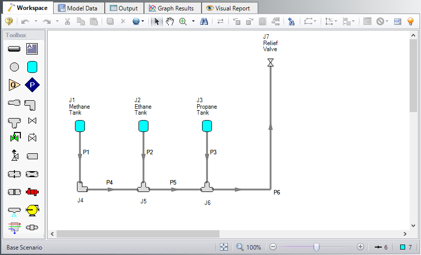
Open the Metric - Refinery Relief System.aro example file listed above, which is located in the Examples folder in the AFT Arrow application folder. Save the file to a different folder. This is the only scenario needed for this example, so right-click the Base Scenario and select Delete All Children. The workspace should look like Figure 1

Step 2. Define the Fluid Properties Group

1. Navigate to the Fluid panel in Analysis Setup

2. Define the Fluid panel with the following inputs

   1. Fluid Library = AFT Standard

   2. Fluid = Steam

      1. After selecting, click Add to Model

   3. Equation of State = Redlich-Kwong

   4. Enthalpy Model = Generalized

   5. Specific Heat Ratio Source = Library

Step 3. Define the Pipes and Junctions Group

All pipes and junctions should already be defined. However, a few changes need to be made to adapt the model to this example. Make the following changes:

Junction Properties

1. J1 Tank

   1. Name = Steam Process 1

   2. Fluid = Steam

   3. Temperature = 205 deg. C

2. J2 Tank

   1. Name = Steam Process 2

   2. Fluid = Steam

   3. Temperature = 205 deg. C

3. J3 Tank

   1. Name = Steam Process 3

   2. Fluid = Steam

   3. Temperature = 205 deg. C

Step 4. Define the Modules Group

Navigate to the Modules panel in Analysis Setup. Check the box next to Activate GSC. The Use option should automatically be selected, making GSC enabled for use.

Step 5. Define the Goal Seek and Control Group

Specify the variables and goals for the model using the Goal Seek and Control group in Analysis Setup.

Variables Panel

Open the Variables panel, click New Variable, and enter the following variable data:

1. Apply = Selected

2. Object Type = Junction

3. Junction Type = Valve

4. Junction Number and Name = J7 (Relief Valve)

5. Variable Parameter = CdA

6. Link To = (None)

7. Lower Bound (Optional) = 0

8. Upper Bound (Optional) = 180

Note: The units used for the Lower and Upper Bound are the same as what is specified in the junction properties window: cm2 in this case.

Goals Panel

Open the Goals panel, click New Goal, and enter the following goal data:

1. Apply = Selected

2. Goal Type = Point

3. Object Type = Pipe

4. Goal Parameter = Mass Flow Rate

5. Criteria = =

6. Goal Value = 13

7. Goal Units = kg/sec

8. Object ID = P6 (Pipe)

9. Object Location = NA

Step 6. Run the Model

Click Run Model on the toolbar or from the Analysis menu. This will open the Solution Progress window. This window allows you to watch as the AFT Arrow solver converges on the answer. Once the solver has converged, view the results by clicking the Output button at the bottom of the Solution Progress window.

Step 7. Examine the Output

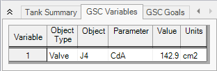
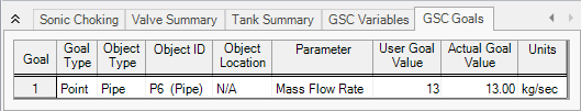
The results of the GSC analysis are shown in the General section of the Output window. The GSC Variables tab shows the final value for the variable parameter, as shown in Figure 2. The GSC Goals tab shows the final value achieved for the goal, as shown in Figure 3.

The GSC module analysis determined that a relief valve CdA value of 142.9 cm2  will result in a relief capacity of 13.00 kg/sec.