Beginner - Pump Sizing for Sand Transfer System - SSL (Metric Units)
Beginner - Pump Sizing for Sand Transfer System - SSL (English Units)
Summary
This example shows how SSL can be used to size a slurry pump as part of a system design process. The piping for a slurry system that moves sand is being designed. The system will pump 25% sand by volume from an open supply vessel with a liquid surface elevation of
Use the SSL module to size the pump.
Note: This example can only be run if you have a license for the SSL module.
Topics Covered
-
Entering solids data
-
Reviewing calculated slurry output
-
Creating slurry system curves
Required Knowledge
This example assumes the user has already worked through the Walk-Through Examples section, and has a level of knowledge consistent with the topics covered there. If this is not the case, please review the Walk-Through Examples, beginning with the Beginner - Three Reservoir example. You can also watch the Fathom Quick Start Video Tutorial Series, as they cover the majority of the topics discussed in the Three-Reservoir Model example.
Model File
This example uses the following file, which is installed in the Examples folder as part of the AFT Fathom installation:
Step 1. Start AFT Fathom
From the Start Menu choose the AFT Fathom 13 folder and select AFT Fathom 13.
To ensure that your results are the same as those presented in this documentation, this example should be run using all default AFT Fathom settings, unless you are specifically instructed to do otherwise.
Step 2. Define the Modules Panel
Open Analysis Setup from the toolbar or from the Analysis menu. Navigate to the Modules panel. For this example, check the box next to Activate SSL and select Settling to enable the SSL module for use. The items in the Fluid Properties group will change to accommodate slurry definitions. Click OK to save the changes and exit Analysis Setup. Open the Analysis menu to see the new option called Slurry. From here you can quickly toggle between Disable mode (normal AFT Fathom) and Settling (SSL mode).
Step 3. Define the Fluid Properties Group
Open Analysis Setup from the toolbar or from the Analysis menu and input the following on the respective panels.
-
Carrier Fluid (Figure 1)
-
Fluid Model = Basic (Water)
-
Temperature = 21 deg. C
-
-
Slurry Definition (Figure 2)
-
Slurry Model = Settling Slurry - Wilson, Addie, Clift
-
Slurry Calculation Method = Detailed
-
Concentration Type = Volume Fraction
-
Amount Solids Added = 25 Percent
-
-
Solids Definition (Figure 3)
-
Solids Specifications = User Specified Solids Added
-
M (Stratification Ratio Exponent) = Calculated
-
Terminal Velocity Parameter, Vt / Vts (Xi) = 1
-
Density = 2.9 S.G. water
-
d50 = 0.0381 cm
-
d85 = 0.0762 cm
-
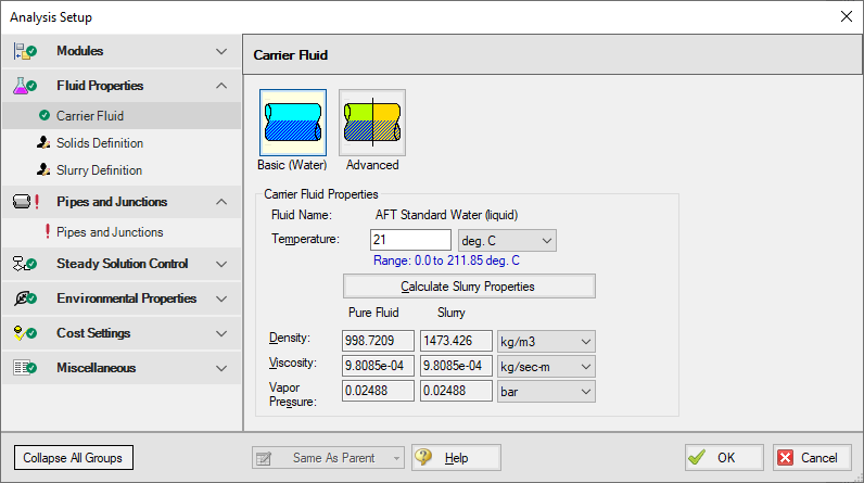
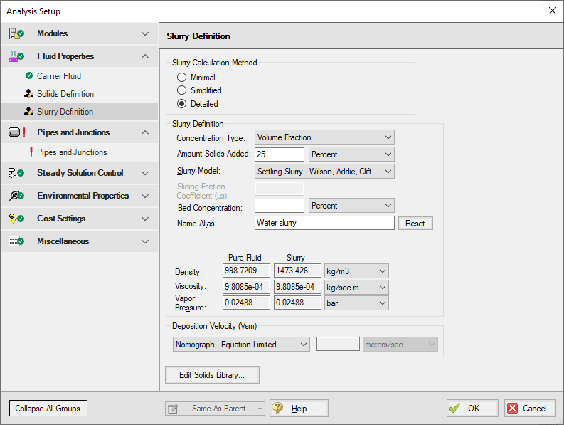
Figure 2: Slurry Definition panel in the Fluid Properties group in Analysis Setup with SSL activated
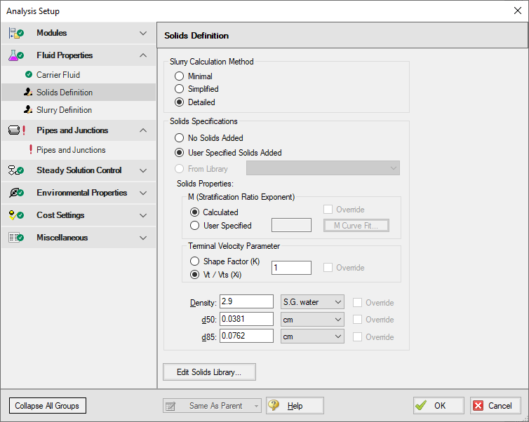
Figure 3: Solids Definition panel in the Fluid Properties group in Analysis Setup with SSL activated
Step 4. Define the Pipes and Junctions Group
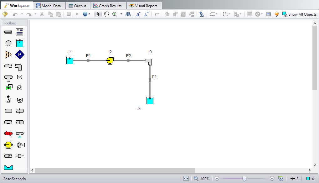
At this point, the first two groups are completed in Analysis Setup. The next undefined group is the Pipes and Junctions group. To define this group, the model needs to be assembled with all pipes and junctions fully defined. Click OK to save and exit Analysis Setup then assemble the model on the workspace as shown in the figure below.
Enter the following pipe and junction properties.
Pipe Properties
-
All Pipes
-
Pipe Material = Steel - ANSI
-
Pipe Geometry = Cylindrical Pipe
-
Size = 12 inch
-
Type = STD
-
Friction Model Data Set = Standard
-
Length =
| Pipe | Length (meters) |
|---|---|
| 1 | 6 |
| 2 | 150 |
| 3 | 15 |
Junction Properties
-
J1 Reservoir
-
Name = Supply Tank
-
Liquid Surface Elevation = 1.5 meters
-
Liquid Surface Pressure = 0.7 barG (70 kPa(g))
-
Pipe Depth = 1.5 meters
-
-
J2 Pump
-
Inlet Elevation = 0 meters
-
Pump Model tab
-
Pump Model = Centrifugal (Rotodynamic)
-
Analysis Type = Sizing
-
Parameter = Mass Flow Rate
-
Fixed Flow Rate = 1270 m-ton/hr Solids
-
-
Slurry De-Rating tab
-
De-Rating Method = ANSI/HI Standard 12.1-12.6-2016
-
Percent Fines = 0 %
-
Head De-Rating Data = Specify Impeller Size Directly
-
Impeller Size = 20 cm
-
-
-
J3 Elbow
-
Inlet Elevation = 0 meters
-
Type = Standard Elbow (knee, threaded)
-
Angle = 90 Degrees
-
-
J4 Reservoir
-
Name = Receiving Tank
-
Liquid Surface Elevation = 3 meters
-
Liquid Surface Pressure = 2 barG (200 kPa(g))
-
Pipe Depth = 3 meters
-
To show the names of the reservoirs, a new Workspace Layer will be created.
-
Create a new layer by selecting New Layer and then Blank Layer from the Workspace Layers tab of the Quick Access Panel.
-
Name the layer Reservoir Labels.
-
Edit the layer by selecting it and clicking the gear icon to bring up the Layer Settings window.
-
Open the Show/Hide Labels panel and uncheck Force Shown Labels to Match Shown Objects.
-
Toggle the visibility icon next to the reservoirs to on. This will cause their labels to be shown.
-
Navigate to the Junction Parameters panel and expand the Commonly Used Junction Parameters list.
-
Double-click Junction Name to add it to the list on the right-hand side. This will add the Junction Name to the label of the junctions that were defined in the Show/Hide Labels panel.
-
Close the Layer Settings window.
ØTurn on Show Object Status from the View menu to verify if all data is entered. If so, the Pipes and Junctions group in Analysis Setup will have a check mark. If not, the uncompleted pipes or junctions will have their number shown in red. If this happens, go back to the uncompleted pipes or junctions and enter the missing data.
Step 5. Run the Model
Click Run Model on the toolbar or from the Analysis menu. This will open the Solution Progress window. This window allows you to watch as the AFT Fathom solver converges on the answer. Now view the results by clicking the Output button at the bottom of the Solution Progress window.
Step 6. Examine the Output
Open the Output Control window by selecting Output Control from the Output toolbar or Tools menu.
On the Display Parameters tab, click the Pumps button, and add the De-rating Head Correction factor (CH) to the Pump Summary output.
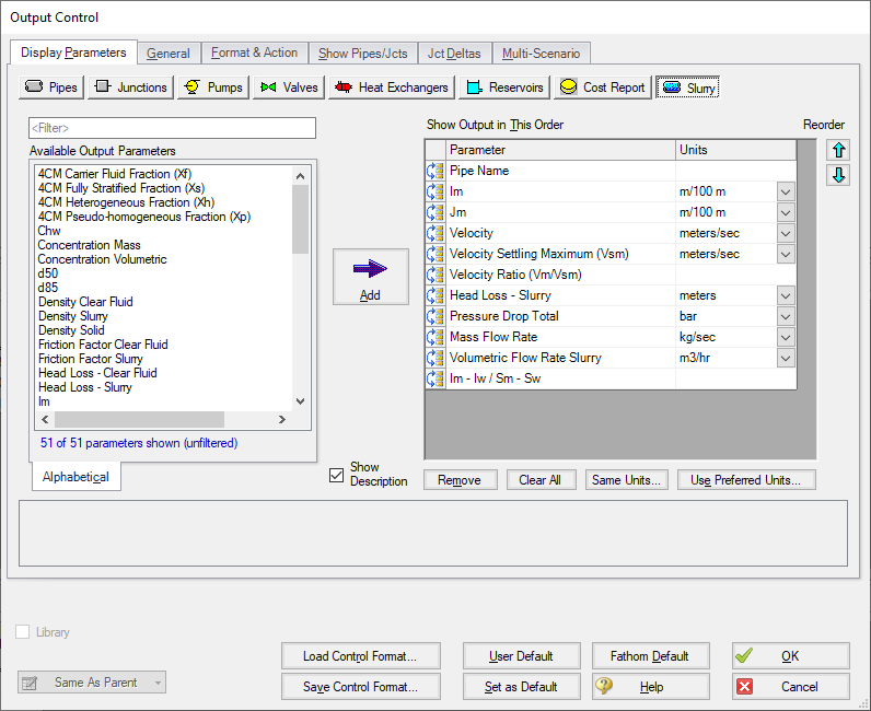
The Output Control window can also be used to configure the slurry output data, as is shown in Figure 5. Click OK when you are finished.
The Slurry tab in the pipes section shows the slurry results, as shown in Figure 6. Here one can see that the velocity is
Also shown in Figure 6 is the Pump Summary in the General Section. There, the required pump head is shown as
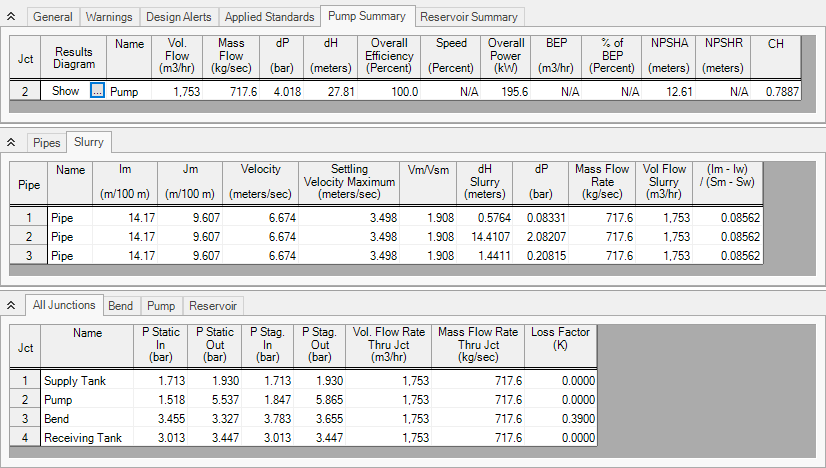
Figure 6: The Output window shows the Slurry results table in the center Pipes section and the pump de-rating in the Pump Summary in the upper General section
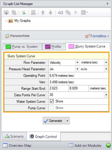
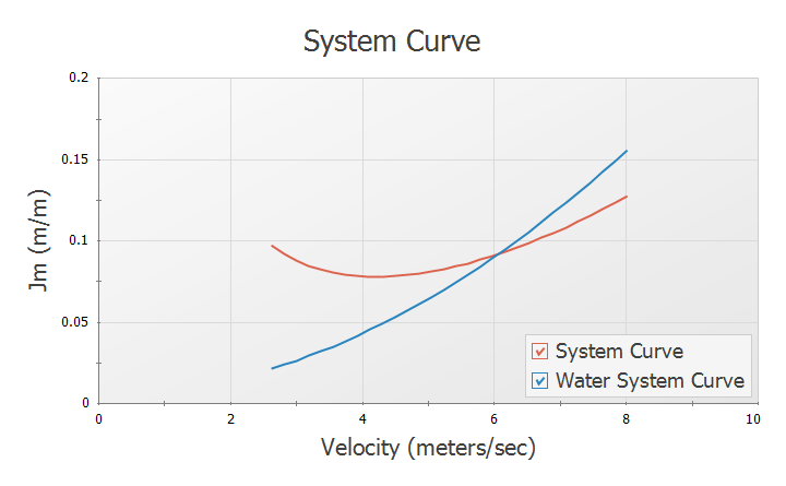
Also of interest is the system curve. Select the Graph Results window tab then in the Graph Control tab in the Quick Access Panel select the Slurry System Curve tab. See Figure 7.
By default the parameter to graph is Jm vs. Velocity. Select the units of Jm as
Conclusion
The pump head requirements were determined, and a de-rating factor was calculated according to the ANSI/HI Standard 12.1-12.6-2016. The de-rating factor for pump head (CH) was used to manually calculate pump head using water, such that the correct size pump could be selected when looking at manufacturer data based on water curves. The velocity in each pipe was found to be higher than the max settling velocity (Vsm) of the sand and water slurry which ensured that no settling would occur. A slurry system curve was created to allow the user to see where the system was operating with respect to solids settling.


