Beginner Valve Closure
(English Units)
Beginner Valve Closure (Metric Units)
Summary
This example is designed to give you the big picture of AFT Impulse's layout and structure. Some of the more basic concepts will be used to build a four pipe, five junction model of the waterhammer transients that result when a valve is closed.
Topics Covered
-
Building a basic model
-
Entering pipe and junction data
-
Entering transient data
-
Graphing output results
Required Knowledge
This example assumes the user has not used AFT Impulse previously. It begins with the most basic elements of laying out the pipes and junctions and solving the transient/waterhammer system hydraulics via the Method of Characteristics (MOC).
Model File
Step 1. Start AFT Impulse
ØTo start AFT Impulse, click Start on the Windows taskbar and open AFT Impulse 9. (This refers to the standard menu items created by setup. You may have chosen to specify a different menu item).
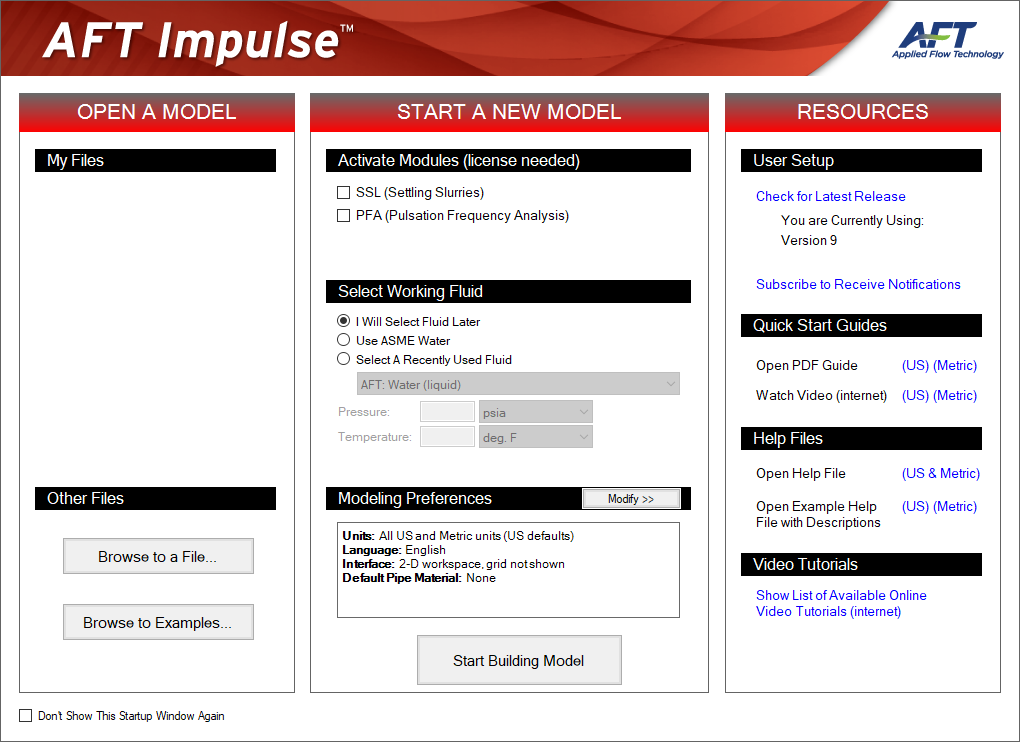
As Impulse is started, the Impulse Startup Window, as shown in Figure 1 appears and provides you with several options before you start building a model. You can open a model that was recently worked on or browse to a different Impulse file or the Impulse Example files. If the Impulse SSL or PFA add-on module is owned, it can be activated here. The Unit System can also be specified to use US Only, Metric Only, Both with US Defaults, or Both with Metric Defaults and they can be set as the user default at this time as well. You can also set the working fluid to AFT Standard Water (liquid) or another recently used AFT fluid. You can click the link to Check for Latest Release to go to the AFT website to see if you have the latest release of AFT Impulse. You can also Subscribe to Receive Notifications of when product maintenance releases are available, receive the AFT newsletter, etc. Finally, you can open the PDF Quick Start Guide, Video Tutorials, the AFT Impulse Help File or Example Help File.
Note: If you are working through the Metric Units version of the Examples, be sure to specify either Metric Only or Both with Metric Defaults as the unit sets and check the box to Set As My Default.
After clicking Start Building Model in the AFT Impulse Startup window, the Workspace window is initially always the active (large) window, as seen in Figure 2. The five tabs in the AFT Impulse window represent the five primary windows. Each Primary Window contains its own toolbar that is displayed directly beneath the Primary Window tabs.
AFT Impulse supports dual monitor usage. You can click and drag any of the five primary window tabs off of the main Impulse window. Once you drag one of the primary windows off of the Impulse window, you can move it anywhere you like on your screen, including onto a second monitor in a dual monitor configuration. To add the primary window back to the main Impulse primary tab window bar, simply click the X button in the upper right of the primary window.
To ensure that your results are the same as those presented in this documentation, this example should be run using all default AFT Impulse settings, unless you are specifically instructed to do otherwise.
The Workspace window
The Workspace window is the primary vehicle for building your model. This window has three main areas: the Toolbox, the Quick Access Panel, and the Workspace itself. The Toolbox is the bundle of tools on the far left.
The Quick Access Panel is on the right. It is possible to minimize the Quick Access Panel by clicking on the thumbtack pin in the upper right of the Quick Access Panel in order to allow for greater Workspace area.
The Workspace takes up the rest of the window.
You will build your pipe flow model on the Workspace using the Toolbox tools. At the top of the Toolbox is the Pipe Drawing Tool and Annotation Tool. The Pipe Drawing tool, on the upper left, is used to draw new pipes on the Workspace. The Annotation tool allows you to create annotations and auxiliary graphics.
Below the two drawing tools are twenty-five icons that represent the different types of junctions available in AFT Impulse. Junctions are objects that connect pipes and also influence the pressure or flow behavior of the pipe system. The twenty-five junction icons can be dragged from the Toolbox and dropped onto the Workspace.
When you pass your mouse pointer over any of the Toolbox tools, a ToolTip identifies the tool's function.
Step 2. Complete the Analysis Setup
ØNext, click Analysis Setup on the Toolbar that runs across the top of the AFT Impulse window. This opens Analysis Setup (see Figure 3). The Analysis Setup contains nine groups (an additional group will display if the PFA module is active). Each group needs to be completed (indicated with a green checkmark next to the group name) before AFT Impulse allows you to run the Solver.
Analysis Setup can also be accessed by clicking on the Status Light on the Quick Access Panel. Once all of the groups in Analysis Setup are defined, the Model Status light in the lower right corner turns from red to green.
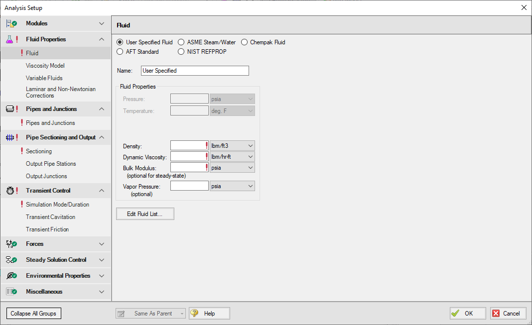
Figure 3: The Analysis Setup tracks the model’s status and allows users to specify required parameters
A. Define the Modules Group
The first group, Modules, will always have a green check when you start AFT Impulse because there are no modules activated by default. No further input is required here.
B. Define the Fluid Properties Group
Next is the Fluid Properties group. This group allows you to specify you fluid properties (density, dynamic viscosity, bulk modulus, and vapor pressure), viscosity model, and fluid corrections. Start by clicking on the Fluid item to open the Fluid panel (see Figure 4).
For models with variable fluid properties, the values for density, viscosity and bulk modulus are default fluid properties. You can then enter different property values, if desired, for any pipe in the Pipe Properties window.
You can model the fluid properties in one of five ways.
-
User Specified Fluid: This fluid model allows you to directly type in the density, viscosity, bulk modulus, and vapor pressure.
-
AFT Standard: This fluid model accesses fluid data from the AFT Standard library. These fluid properties are either temperature dependent or dependent on the solids concentration. Type in the desired condition (e.g., temperature) and the required properties are calculated. Users can add their own fluids to this library. Custom fluids are created by opening the Fluid Library window from the AFT Impulse Library menu or by clicking the Edit Fluid List button at the bottom of the Fluid panel.
-
ASME Steam/Water: As its name implies, this fluid model calculates water properties from the built-in ASME Steam Tables. This model is pressure and temperature dependent.
-
NIST REFPROP: This fluid model allows you to select a single fluid or create a mixture of fluids from the REFPROP fluid library. These fluid properties are pressure and temperature dependent.
-
Chempak Fluid: This fluid model allows you to select a single fluid or create a mixture of fluids from the Chempak fluid library. These fluid properties are pressure and temperature dependent, although some are temperature dependent only. Chempak is an optional add-on to AFT Impulse.
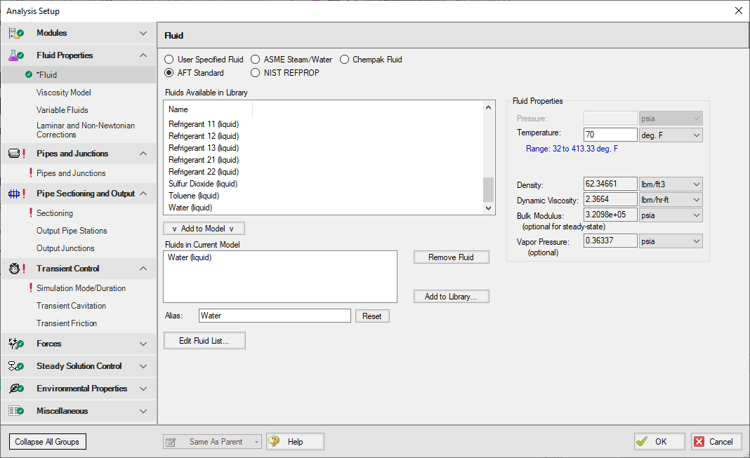
ØSelect AFT Standard, by clicking the radio button next to the name. Then choose Water (liquid) from the list and click Add to Model. The properties for AFT Standard water are given only as a function of temperature. Enter
ØCheck the groups on the left side of Analysis Setup and you should now see the second group is checked off.
On the Viscosity Model panel, users can specify how AFT Impulse will treat viscosity. By default, Newtonian is the viscosity model selected. AFT Impulse offers a variety of non-Newtonian models. However, for this example, the default selection will suffice.
On the Variable Fluids panel, users can specify constant or variable fluid properties. For models with variable fluid properties, the values for density and viscosity are default fluid properties. You can then enter different property values, if desired, for any pipe in the Pipe Properties window. By default, Constant Fluid Properties is selected.
On the Laminar and Non-Newtonian Corrections panel, users can specify the type of corrections that the solver will apply when flow is laminar or if a non-Newtonian viscosity model is selected. The default selections are applicable for most cases, so no input is required for this example.
C. Define the Pipes and Junctions Group
In order to fully define this group, there needs to be pipes and junctions on the Workspace. To lay out the valve closure model, you will place the three reservoir junctions, a valve junction, and a branch junction on the Workspace. Then you will connect the junctions with pipes.
To go back to the Workspace and save the inputs made in Analysis Setup, click OK.
I. Place the first reservoir
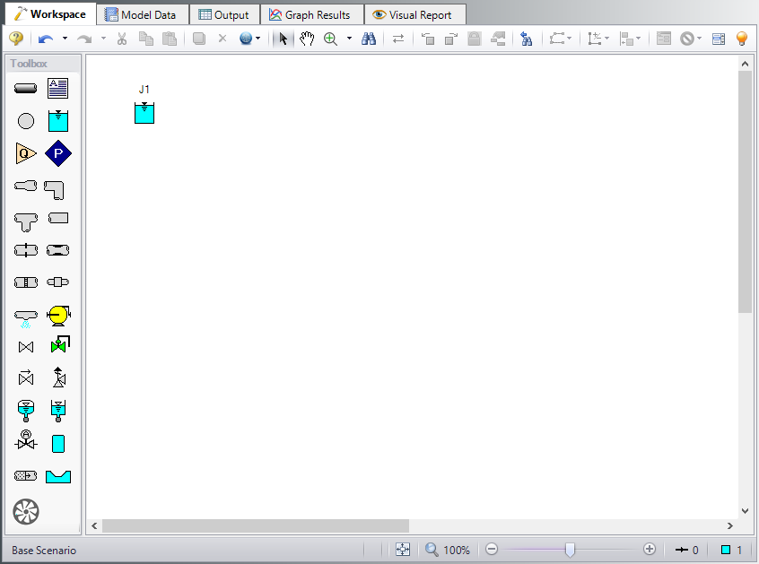
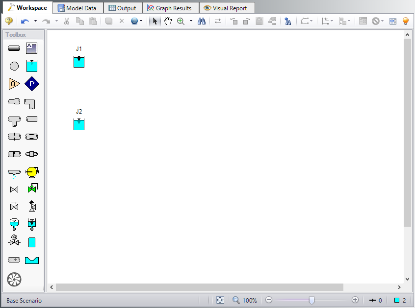
ØTo start, drag a reservoir junction from the Toolbox and drop it on the Workspace. Figure 5 shows the Workspace with one Reservoir.
Objects and ID numbers
Items placed on the Workspace are called objects. All objects are derived directly or indirectly from the Toolbox. AFT Impulse uses three types of objects: pipes, junctions, and annotations.
All pipe and junction objects on the Workspace have an associated ID number. For junctions, this number is, by default, placed directly above the junction and prefixed with the letter J. Pipe ID numbers are prefixed with the letter P. You can optionally choose to display either or both the ID number and the name of a pipe or junction. You also can drag the ID number/name text to a different location to improve visibility.
The reservoir you placed on the Workspace will take on the default ID number of 1. You can change this to any desired number greater than zero and up to 99,999.
Editing on the Workspace
Once on the Workspace, junction objects can be moved to new locations and edited with the features on the Edit menu. Cutting, copying, and pasting are all supported. Multiple levels of undo are available for most editing operations.
Note:: The relative location of objects in AFT Impulse is not important. Distances and heights are defined through dialog boxes. The relative locations on the Workspace establish the connectivity of the objects, but have no bearing on the actual length or elevation relationships.
II. Place the second reservoir
The second reservoir can be created the same way as the first one or can be derived from the existing reservoir.
ØTo create a second reservoir from the existing one, select junction J1 by clicking it with the mouse. A red outline will surround the junction to show it is selected. Choose Duplicate from the Edit menu (or use CTRL+D on the keyboard). Your Workspace should appear similar to that shown in Figure 6.
If you like, you can Undo the Duplicate operation and then Redo it to see how these editing features work. To undo an operation, click on the undo button on the Toolbar or choose Undo from the Edit menu. To redo an operation, choose Redo from the Edit menu.
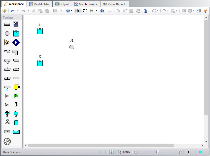
III. Place a Branch junction
ØTo add a Branch junction, select a Branch from the Toolbox and place it on the Workspace as shown in Figure 7. The Branch will be assigned the default number J3.
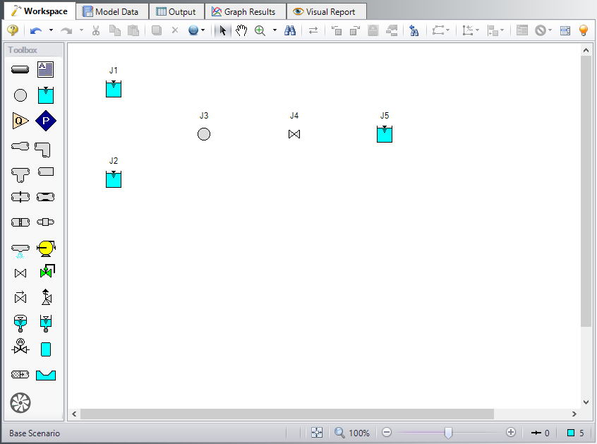
IV. Place a valve and a final reservoir junction
ØTo add a valve junction, click and drag a Valve junction from the Toolbox and place it on the Workspace as shown in Figure 8. The Valve will be assigned the default number J4. Add a third Reservoir junction, number J5, also shown in Figure 8.
ØBefore continuing, save the work you have done so far. Choose Save As from the File menu and enter a file name (Valve Closure, perhaps) and AFT Impulse will append the .imp extension to the file name.
V. Draw a pipe between J1 and J3
Now that you have five junctions, you need to connect them with pipes.
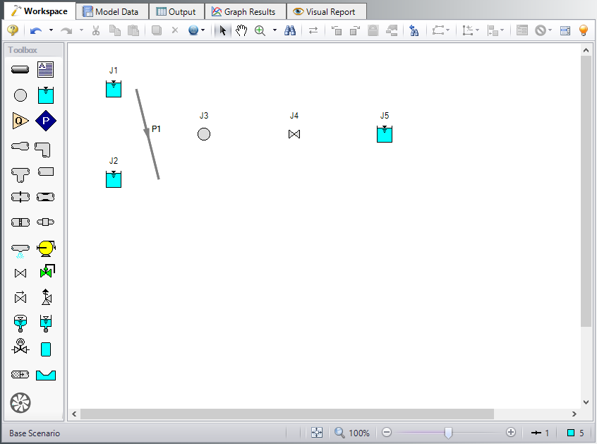
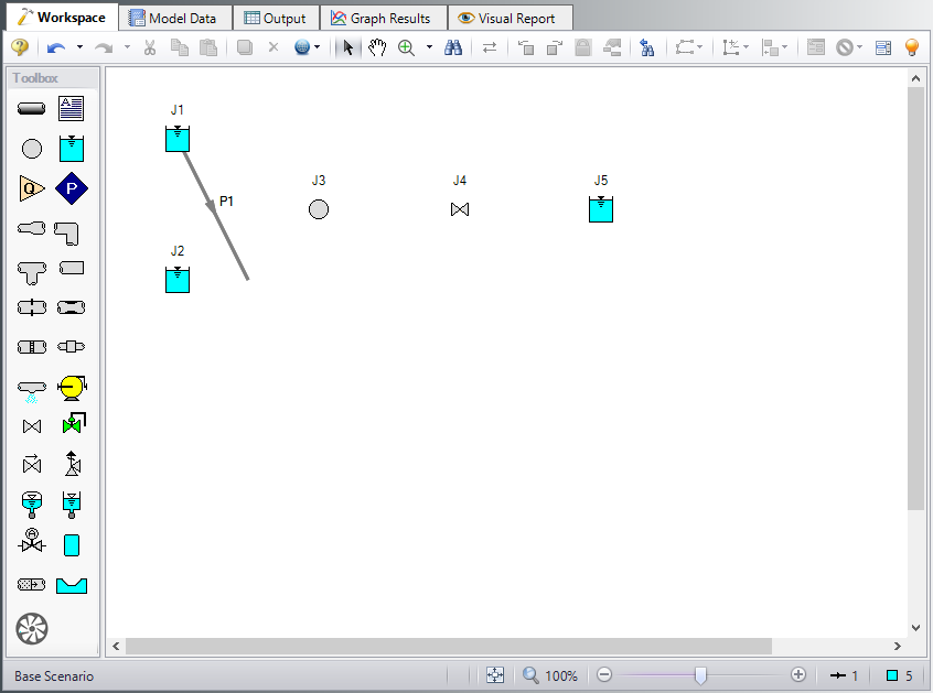
ØTo create a pipe, click the Pipe Drawing tool icon. The pointer will change to a crosshair when you move it over the Workspace. Draw a pipe above the junctions, similar to that shown in Figure 9.
The pipe object on the Workspace has an ID number (P1), shown near the center of the pipe.
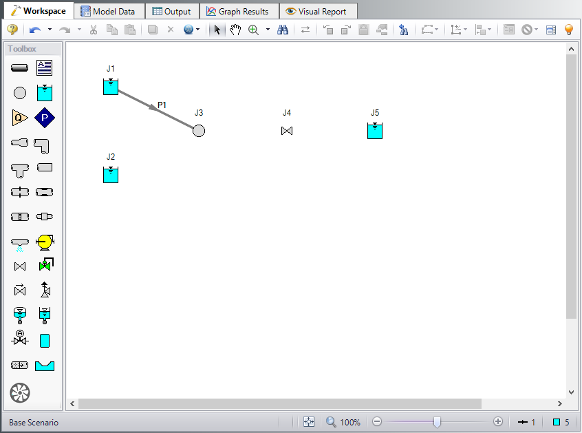
ØTo place the pipe between J1 and J3, use the mouse to grab the pipe in the center, drag it so that its left endpoint falls within the J1 Reservoir icon, then drop it there (see Figure 10). Next, grab the right endpoint of the pipe and stretch the pipe, dragging it until the endpoint terminates within the J3 Branch icon (see Figure 11).
Reference positive flow direction
Located on the pipe is an arrow that indicates the reference positive flow direction for the pipe. AFT Impulse assigns a flow direction corresponding to the direction in which the pipe is drawn. You can reverse the reference positive flow direction by choosing Reverse Direction from the Arrange menu or selecting the reverse direction button on the Workspace Toolbar.
The reference positive flow direction indicates which direction is considered positive. If the reference positive direction is the opposite of that obtained by the Solver, the output will show the flow rate as a negative number.
VI. Add the remaining pipes
A faster way to add a pipe is to draw it directly between the desired junctions.
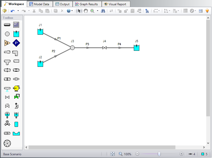
ØActivate the pipe drawing tool again. Position the cursor on the J2 Reservoir. Press and hold the left mouse button. Stretch the pipe up to the J3 Branch then release the mouse button. Then draw a third pipe from the J3 Branch to the J4 Valve. Finally, draw a fourth pipe from the J4 Valve to the J5 Reservoir. Your model should now look similar to Figure 12.
At this point all the objects in the model are graphically connected. Save the model by selecting Save from the File menu or by clicking the Save button on the Toolbar.
Note: It is generally desirable to lock your objects to the Workspace once they have been placed. This prevents accidental movement and disruption of the connections. Locking also helps prevent accidental deletion of your output once a solution has been completed. You can lock all the objects by choosing Select All from the Edit menu, then selecting Lock Object from the Arrange menu. The Lock Object button on the Workspace Toolbar will appear depressed indicating it is in an enabled state, and will remain so as long as any selected object is locked.
VII. Define the pipes and junctions
To fully define the Pipes and Junctions Group in Analysis Setup, all pipes and junctions must be connected and have the proper input data.
Object status
Every pipe and junction has an object status. The object status tells you whether the object is defined according to AFT Impulse's requirements. To see the status of the objects in your model, click the floodlight on the Workspace Toolbar (alternatively, you could choose Show Object Status from the View menu). Each time you click the floodlight, Show Object Status is toggled on or off.
When Show Object Status is on, the ID numbers for all undefined pipes and junctions are displayed in red on the Workspace. Objects that are completely defined have their ID numbers displayed in black. (These colors are configurable through User Options from the Tools menu.)
Because you have not yet defined the pipes and junctions in this model, all the objects' ID numbers will change to red when you turn on Show Object Status.
Undefined Objects window
The Undefined Objects window lists all undefined pipes and junctions and further displays the items that are not yet defined.
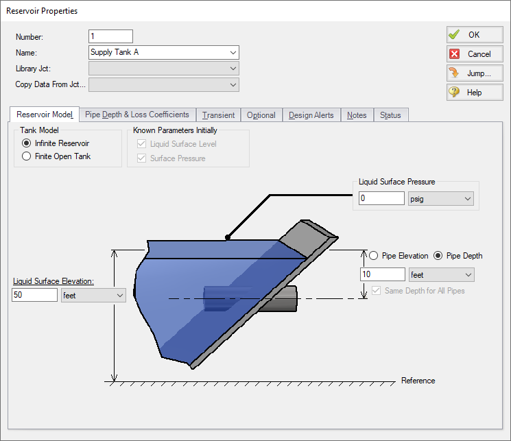
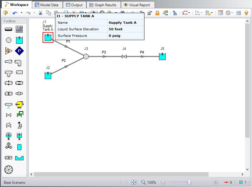
VIII. Define Reservoir J1
ØTo define the reservoir J1, open the J1 Reservoir Properties window (see Figure 13) by double-clicking the J1 icon. By default you will begin on the Reservoir Model tab. For Tank Model make sure Infinite Reservoir is selected. Enter a Liquid Surface Elevation of
Note: You can also open an object's properties window by selecting the object (clicking on it) and then either pressing the Enter key or clicking the Open Pipe/Jct Window icon on the Workspace Toolbar.
ØEnter a Liquid Surface Pressure of 0 psig and with Pipe Depth selected, enter
Note: You can specify preferred units for many parameters (such as meters for length) in the User Options from the Tools menu.
You can give the object a name, if desired, by entering it in the Name field at the top of the window. In Figure 13, the name of this reservoir is Supply Tank A. By default the junction’s name is the junction type. The name can be displayed on the Workspace, Visual Report or in the Output.
Most junction types can be entered into a custom library allowing the junction to be used multiple times or shared between users. To select a junction from the custom library , choose the desired junction from the Library Jct list. The current junction will get the properties from the library.
The Copy Data From Jct list will show all the junctions of the same type in the model. This will copy all the parameters from an existing junction in the model to the current junction.
The pipe table on the Pipe Depth & Loss Coefficients tab allows you to specify entrance and exit loss factors for each pipe connected to the reservoir (in this case there is one). You can enter standard losses by selecting the option buttons at the right. The default selection is the Custom option with loss factors specified as zero. To later change the loss factors, click within the pipe table and enter the loss. You can also specify a depth for the pipe.
The Transient tab can be used to specify how the liquid surface elevation changes with time.
The Optional tab allows you to enter different types of optional data. You can select whether the junction number, name, or both are displayed on the Workspace. Some junction types also allow you to provide a guess for initial pressure as well as other junction specific data. The junction icon graphic can be changed, as can the size of the icon. Design factors can be entered for most junctions, which are applied to the pressure loss calculations for the junction in order to give additional safety margin to the model.
The Design Alerts tab shows the design alerts that are applied to the junction, which ensures that the model is behaving as expected.
The Notes tab allows you to enter text describing the junction or documenting any assumptions.
The Status tab lists the remaining undefined items for the junction. It should show that All Items Defined.
The highlight feature displays all the required information in the properties window in light blue. The highlight is on by default. You can toggle the highlight off and on by double-clicking anywhere in the window or by pressing the F2 key. The highlight feature can also be turned on or off in the User Options window from the Tools menu. All examples images will be shown with this highlight option turned off.
ØClick OK. You may be prompted to display the junction name on the Workspace, if so, click Yes. If Show Object Status is turned on, you should see the J1 ID number turn black again, telling you that J1 is now completely defined.
The Inspection feature
You can check the input parameters for J1 quickly, in read-only fashion, by using the Inspection feature. Position the mouse pointer on J1 and hold down the right mouse button. An information box appears, as shown in Figure 14.
Inspecting is a fast way of examining the input (and output if output results are available) for an object.
IX. Define Reservoir J2
ØNext, open the properties window for reservoir J2 and make sure the Tank Model selection is Infinite Reservoir, then enter a Liquid Surface Elevation of
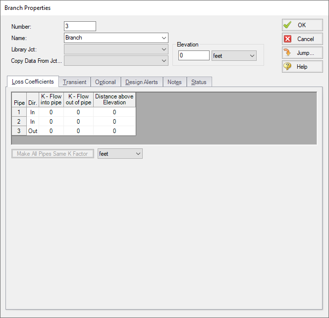
X. Define Branch J3
ØOpen the properties window for branch J3 (see Figure 15). In this window, all three connecting pipes should be displayed in the pipe table area. You could associate loss factors with each pipe by clicking within the pipe table and entering the data. Enter an elevation of 0
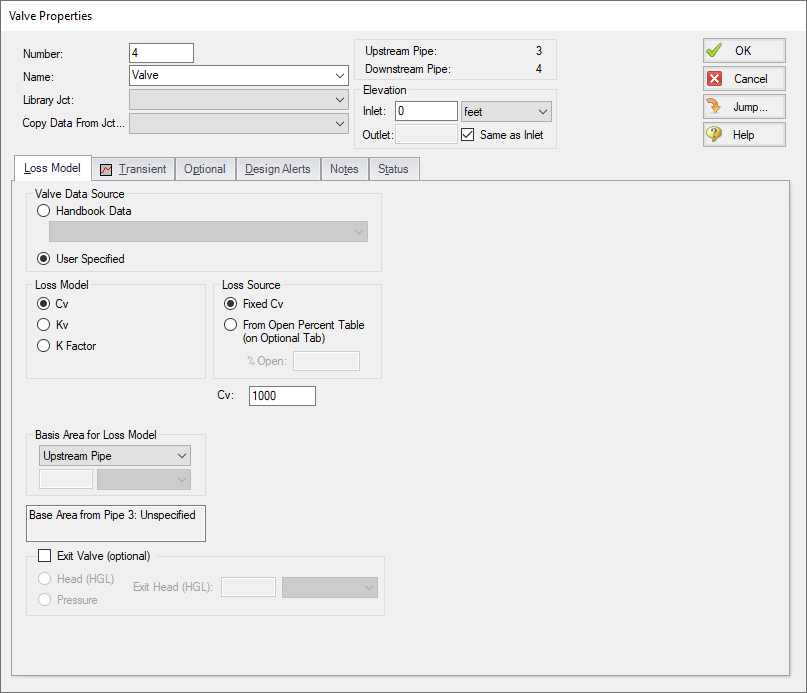
XI. Define Valve J4
ØOpen the properties window for valve J4 (see Figure 16) and enter an Inlet Elevation of 0
ØOn the Loss Model tab, make sure the Valve Data Source has User Specified selected.
ØFor Loss Model, make sure Cv is selected and enter a Cv value of 1000. This represents the valve's Cv during steady-state.
ØClick the Transient tab and enter the data below for Cv (see Figure 17).
| Time (seconds) | Cv |
|---|---|
| 0 | 1000 |
| 0.4 | 400 |
| 0.8 | 100 |
| 1 | 0 |
| 2 | 0 |
The first data point (Cv = 1000 at time zero) must match the steady-state value. The transient data represents the valve initially open. The valve then gradually closes over a period of one second, and stays closed.
The J4 Valve is the element which causes the transient in this model. The purpose of the model will be to understand how high the pressures can rise during the transient.
When transient data is entered for a junction, a T symbol is shown next to the junction number on the Workspace.
XII. Define reservoir J5
ØFinally, open the properties window for reservoir J5 and make sure the Tank Model selection is Infinite Reservoir, then enter a Liquid Surface Elevation of
ØSave the model again before proceeding.
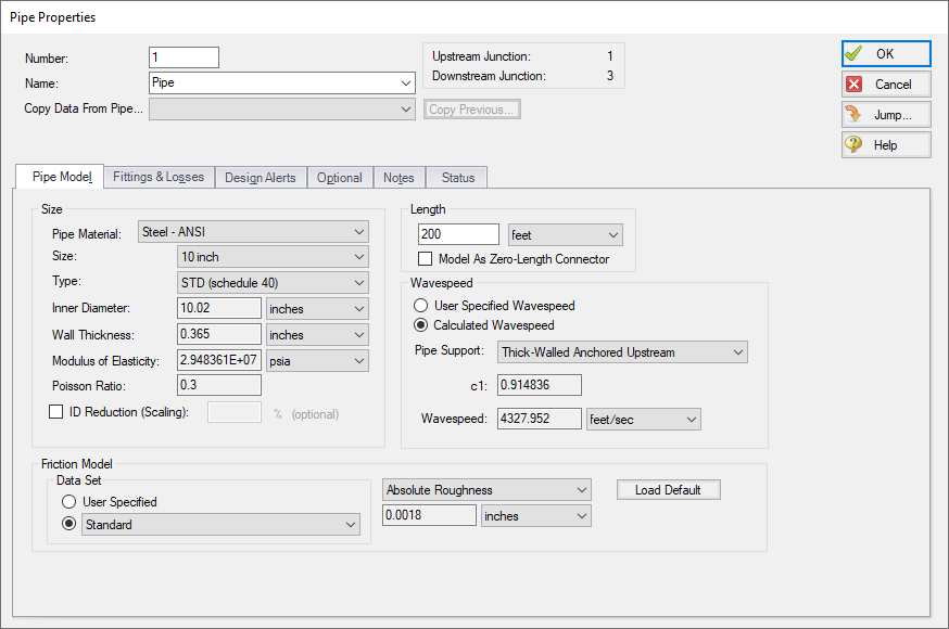
XIII. Define pipe P1
The next step is to define all the pipes. To open the Pipe Properties window, double click the pipe on the Workspace.
ØFirst open the Pipe Properties window for Pipe P1 (see Figure 18). For Pipe P1, enter a length of
The wavespeed is a very important parameter in a waterhammer analysis. The wavespeed can be calculated with reasonable accuracy from fluid and pipe data, or it may be available from test data or industry publications. If the wavespeed is not known (which is typical), then the Calculated Wavespeed option is preferred option. In this case, data is required for pipe wall thickness, modulus of elasticity, Poisson Ratio, and pipe support details. Data for pipe wall thickness, modulus of elasticity, Poisson Ratio are built into the pipe material libraries supplied with AFT Impulse, and is automatically obtained when the pipe material, size, and type are chosen. The calculated wavespeed is
The Pipe Properties window offers control over all important flow system parameters that are related to pipes. Click OK.
The Inspect feature also works within the Pipe Properties window. To inspect a connected junction, position the mouse pointer on the connected junction's ID number and hold down the right mouse button. This is helpful when you want to quickly check the properties of connecting objects. (You can also use this feature in junction Properties windows for checking connected pipe properties.)
By double-clicking the connected junction number, you can jump directly to the junction's Properties window. Or you can click the Jump button to jump to any other part of your model.
XIV. Define pipes P2, P3, and P4
Define pipes P2 - P4 as Steel - ANSI using the sizes and lengths shown below. All pipes should use Thick-Walled Anchored Upstream for the Pipe Support model.
The data for the pipes should be as follows:
| Pipe | Size (inches) | Length (feet) |
|---|---|---|
| 1 | 10 | 200 |
| 2 | 10 | 150 |
| 3 | 12 | 50 |
| 4 | 12 | 40 |
After entering the data for all the pipes, the Pipes and Junctions Group should be completed. If it is not, see if the Show Object Status is on. If it is not turned on, select Show Object Status from the View menu or Workspace Toolbar. If the Pipes and Junctions Group in Analysis Setup does not have a green checkmark next to it, see if any of the pipes or junctions have their number displayed in red. If so, you did not enter all the data for that item.
ØBefore running the model, save it one more time. It is also a good idea to review the input using the Model Data window.
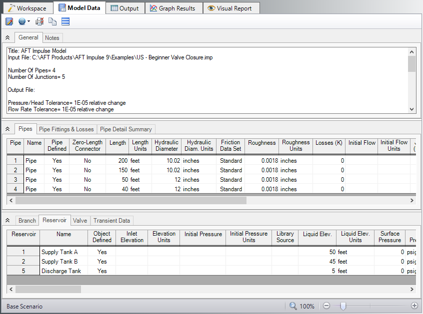
Reviewing input in the Model Data window
The Model Data window is shown in Figure 19. To change to this window, you can select it from the Primary Window tabs or the Window menu, or by pressing CTRL+M. The Model Data window gives you a text based perspective of your model. Selections can be copied to the clipboard and transferred into other Windows programs, or printed out for review. Figure 20 shows an expanded view of the Transient Data tab from Figure 19. Here all transient input data for the model is shown.
The Model Data window allows access to all Properties windows by double-clicking anywhere in the row associated with the appropriate ID number in the far left column of the table. You may want to try this right now.
D. Define the Pipe Sectioning and Output Group
After completing the first three Analysis Setup Groups, sufficient information exists to run the model in steady-state. The next two groups are for transient modeling. To run the model in steady-state, open the Analysis menu, select Time Simulation, then choose Steady Only. By doing this, the final two Checklist items are grayed out and the model can be run.
In general, it is a good idea to always run your model in steady-state first before running the full transient analysis to make sure the model is giving reasonable results.
The Pipe Sectioning and Output group allows the user to define pipe sectioning and how much information to save to the output file.
I. Define the Sectioning Panel
The only item in the Pipe Sectioning and Output Group in Analysis Setup that needs user input is the Sectioning panel. This panel cannot be defined until the Fluid Properties group and Pipes and Junctions group are defined. The Sectioning panel divides the pipes into computation sections in a manner which is consistent with the Method of Characteristics (MOC).
ØOpen the Sectioning panel in Analysis Setup (Figure 21). The pipes will automatically be sectioned without user input. For this model the controlling pipe is P4. This is the pipe with the shortest end-to-end communication time (i.e., L/a – the length divided by the wavespeed). To satisfy the MOC, the following equation must be applied:

where n is the number of sections in pipe i, L is the length, and a is the wavespeed. The Dt is the time step. Since all pipes in the network must be solved together, the same time step must be used for each pipe. With a given length and wavespeed for each pipe, it can be seen from the above equation that it is unlikely that the number of required sections, n, for each pipe will be a whole number.
To address this situation, it is helpful to recognize that the wavespeed, a, is the least certain input parameter. It is therefore commonly acceptable to allow up to a 15% uncertainty in wavespeed, though AFT Impulse by default only allows up to 10% variance. By adjusting the wavespeed for each pipe within this tolerance the sectioning can be made to come out as whole numbers for each pipe. The Section Pipes window automates this process by searching for sectioning which satisfies the required tolerance.
You can customize the Section Pipes search criteria by clicking the arrow next to Advanced Settings. In general, the default search criteria will be sufficient for adequately sectioning the pipes throughout your model.
In this example, make sure the second row that will use two pipe sections in the controlling pipe is selected. The Sectioning Panel and Pipe Sectioning and Output group should now have a green checkmark indicating that they are fully defined.
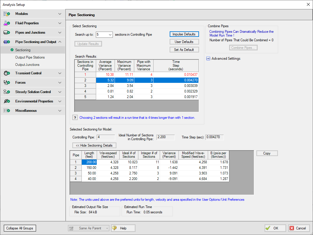
Figure 21: The Sectioning Panel automates the sectioning process and calculates the time step
E. Define the Transient Control Group
The final Analysis Setup group to define is the Transient Control Group. This group allows you to specify the time at which the transient starts and ends, the cavitation model used, and the friction method used.
ØOpen the Simulation Mode/Duration panel in Analysis Setup (Figure 22). Zero (0) seconds should already be entered for Start Time. Enter two (2) for Stop Time.
The Transient Cavitation panel allows you to enable or disable transient cavitation modeling. It is advised to keep Model Transient Cavitation checked and only disable it for troubleshooting purposes.
Note: The Artificial Transient Detection panel in the Miscellaneous group offers control over how AFT Impulse should respond to artificial transients. Artificial transients are a problem that can sometimes occur when steady-state and initial transient conditions are inconsistent.
At the bottom of the panel the projected output file size is shown. You should pay attention to this number, as the output file size can grow very large. In this case the output file will be
ØClick OK to accept the current settings now that all groups are defined. The model is ready to be solved.
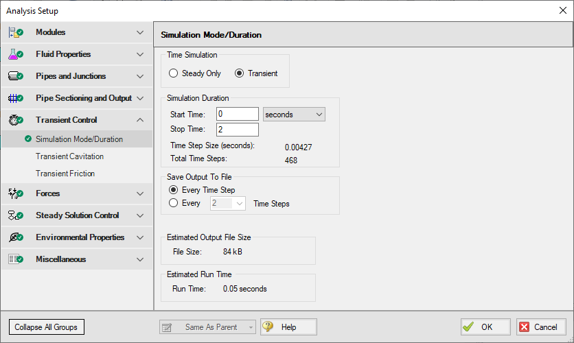
Figure 22: The Simulation Mode/Duration panel offers features to specify the time span for the transient and what output data is written
Step 3. Run the Solver
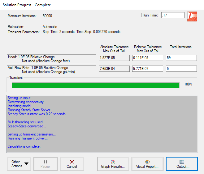
ØClick Run Model from the toolbar or from the Analysis menu. During execution, the Solution Progress window displays (Figure 23). You can use this window to pause or cancel the Solver's activity.
The Two Solvers
AFT Impulse has two solvers. The first is called the Steady-State Solver, which as its name suggests obtains a steady-state solution to the pipe network. The second solver is called the Transient Solver. This solves the waterhammer equations.
Before a transient simulation can be initiated, the initial conditions are required. These initial conditions are the steady-state solution to the system. After the steady-state solution is obtained by the Steady-State Solver, AFT Impulse uses the results to automatically initialize the Transient Solver and then run it.
ØWhen the solution is obtained, click the Output button to display the text-based Output window. The information in the Output window can be reviewed visually on the screen, saved to file, exported to a spreadsheet-ready format, copied to the clipboard, and printed out on the printer.
The transient output file
When the Transient Solver runs, the transient output data is written to a file. This file is given the same name as the model itself with a number appended to the name, and with an .out extension appended to the end. For all transient data processing, graphing, etc., the data is extracted from this file. The number is appended because AFT Impulse allows the user to build different scenarios all within this model. Each scenario will have its own output file, thus the files need to be distinguishable from each other.
The output file will remain on disk until the user erases it or the model input is modified. This means that if you were to close your model right now and then reopen it, you could proceed directly to the Output window for data review without rerunning your model.
Step 4. Examine the Output
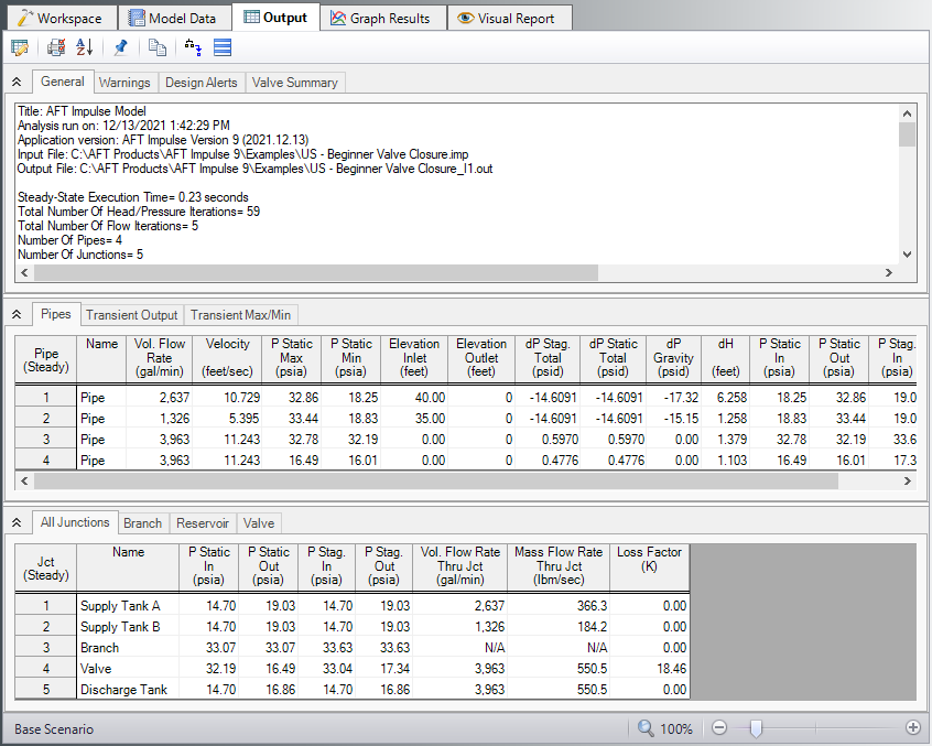
The Output window (Figure 24) is similar in structure to the Model Data window. Three areas are shown, and you can minimize or enlarge each section by clicking the arrow next to the General, Pipes, and All Junctions tabs or from the View menu. The parameters displayed in the tables can be customized with the Output Control window, from the Tools drop-down menu.
The Output window allows you to review both the steady-state and transient results. You can review the solutions for each time step (i.e., a time history) for which data was written to file. Also, a summary of the maximum and minimum transient results for each computing station is given on the Transient Max/Min tab in the pipe area. These two data sets are located on the Transient Output tab and Transient Max/Min tab in the pipe area of the Output window (see Figure 25 and Figure 26). Note that in order to display all pipe stations as shown in Figure 25, the model will need to be set to save data for all stations. By default, AFT Impulse will only save the inlet and outlet data points for each pipe. This can be changed on the Output Pipe Stations Panel in the Pipe Sectioning and Output Group in Analysis Setup.
A. Modify the output format
If you selected the default AFT Impulse Output Control, the Pipes table of steady-state results (the tab on the far left in the pipe area) will show volumetric flow rate in the second column with units of
ØSelect Output Control from the Tools menu or the main Toolbar. On the right side of the Pipes section is the list of currently selected output parameters. Click Volumetric Flow Rate and change the units by clicking the arrow beside the units, and then selecting
ØClick OK to display changes to the current results. You should see the volumetric flow rate results, still in the second column, in units of
ØSelect Output Control from the Tools menu one more time. The Reorder scroll bar on the far right allows you to reorder parameters in the list. You may also reorder parameters by dragging and dropping the icon just to the left of each parameter within the list of currently selected parameters.
ØSelect the Velocity parameter and use the Reorder scroll bar to move it up to the top of the parameter list.
ØClick OK to display the changes to the current results. You will see in the Pipes table that the first column now contains velocity and the third column contains the volumetric flow rate. The Output Control window allows you to obtain the parameters, units and order you prefer in your output. This flexibility will help you work with AFT Impulse in the way that is most meaningful to you, reducing the possibility of errors.
ØLastly, double-click the column header Velocity in the Output window Pipes Table. This will open a window in which you can change the units once again if you prefer. These changes are extended to the Output Control parameter data you have previously set.
B. Graph the results
For transient analyses, the Graph Results window will usually be more helpful than the Output window because of the more voluminous data.
ØBrowse to the Graph Results window by clicking the Graph Results tab, choosing it from the Windows menu, or by pressing CTRL+G. The Graph Results window offers full-featured Windows plot preparation.
The Graph Parameters menu will automatically be displayed in the Quick Access Panel on the far right of the Graph Results Window, and be where you are to specify which graphs to generate. On the Transient Pipe tab under Select Pipe Stations, expand P3 pipe stations and double-click Outlet, which is the pipe computing station at the valve inlet. Also add the inlet of pipe P4 which is the valve exit. Select the Graph Parameter as Pressure Static and set the units to
ØClick Generate. The graph shows the static pressure at the valve inlet and outlet over the duration of the simulation (See Figure 28).
You can use the other buttons in the Graph Results window to change the graph appearance and to save and import data for cross-plotting. The Graph Results window can be printed, saved to file, copied to the clipboard, or printed to an Adobe PDF file. The graph's x-y data can be exported to file or copied to the clipboard.
Note that the graph guide, located at the top right of the Graph Results window and represented with the What Would You Like to Do? icon, can guide you through the development of your graph. This feature can be hidden by clicking on the icon.
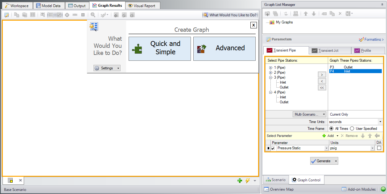
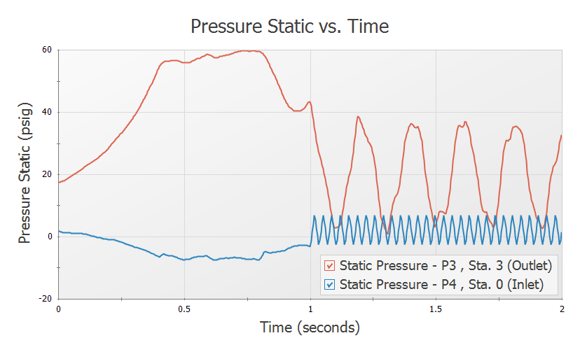
Figure 28: The Graph Results window offers full-featured plot generation. Here the static pressure at valve J4 over time is shown
Further review of the valve graph results in Figure 28 shows that at time zero the difference between the curves is about
As time increases one sees that the pressure drop across the valve increases as it closes. Finally at 1 second, the valve closes entirely and the pipes upstream and downstream of the valve are isolated from each other and will decay to the steady-state conditions which exist for a closed valve.
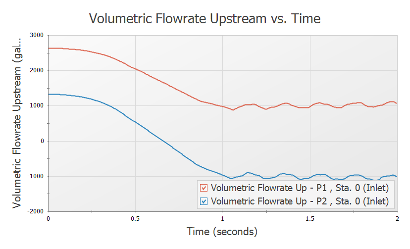
In the Graph Parameters window on the Quick Access Panel click ![]() (Clear button). Expand Pipe 1 and select the Inlet of Pipe 1 by double-clicking or clicking the Add button. This is the pipe computing station at the reservoir J1. Also add the inlet of Pipe 2 which is the reservoir J2. Select the Graph Parameter as Volumetric Flowrate Upstream and set the units to
(Clear button). Expand Pipe 1 and select the Inlet of Pipe 1 by double-clicking or clicking the Add button. This is the pipe computing station at the reservoir J1. Also add the inlet of Pipe 2 which is the reservoir J2. Select the Graph Parameter as Volumetric Flowrate Upstream and set the units to
C. View the Visual Report
ØChange to the Visual Report window by choosing it from the Window menu, clicking the Visual Report tab on the toolbar, or by pressing CTRL+I. This window allows you to integrate your text results with the graphic layout of your pipe network. The Visual Report can also animate the transient pipe results in a color animation overlaid on the model.
ØThe Visual Report Control window should open automatically shown in Figure 30. Default parameters are already selected, but you can modify these as desired. For now, in the Pipe Transient Output area, select Max Pressure Stagnation and Min Pressure Stagnation. Click the Show button. The Visual Report window graphic is generated (see Figure 30).
It is common for the text in the Visual Report window to overlap when first generated. You can change this by selecting smaller fonts or by dragging the text to a new area to increase clarity (this has already been done in Figure 31). This window can be printed or copied to the clipboard for import into other Windows graphics programs.
The Visual Report window also provides the ability to animate the transient results as a qualitative tool to visualize the behavior in a network. This option can also be accessed from the Visual Report Control by selecting the Animate under Display Mode at the top of the Visual Report Control window (See Figure 30). When using the animation mode, text results cannot be displayed for the report. Instead, one parameter can be animated using absolute values or values relative to the steady state, or a static map of all maximum/minimum transient values can be generated. The animation can be recorded to a file. The model setup for animating pressure stagnation can be seen in Figure 32.
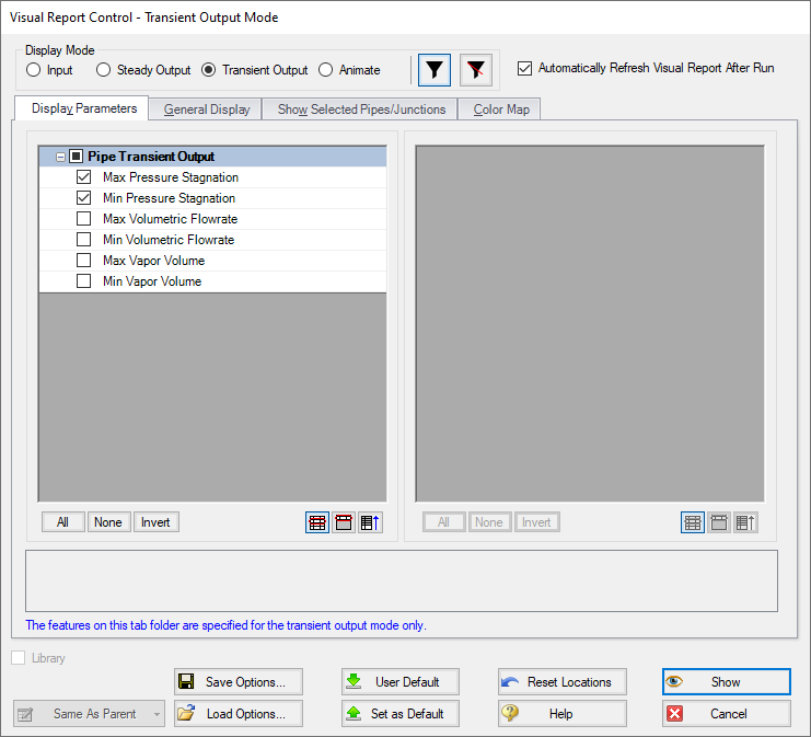
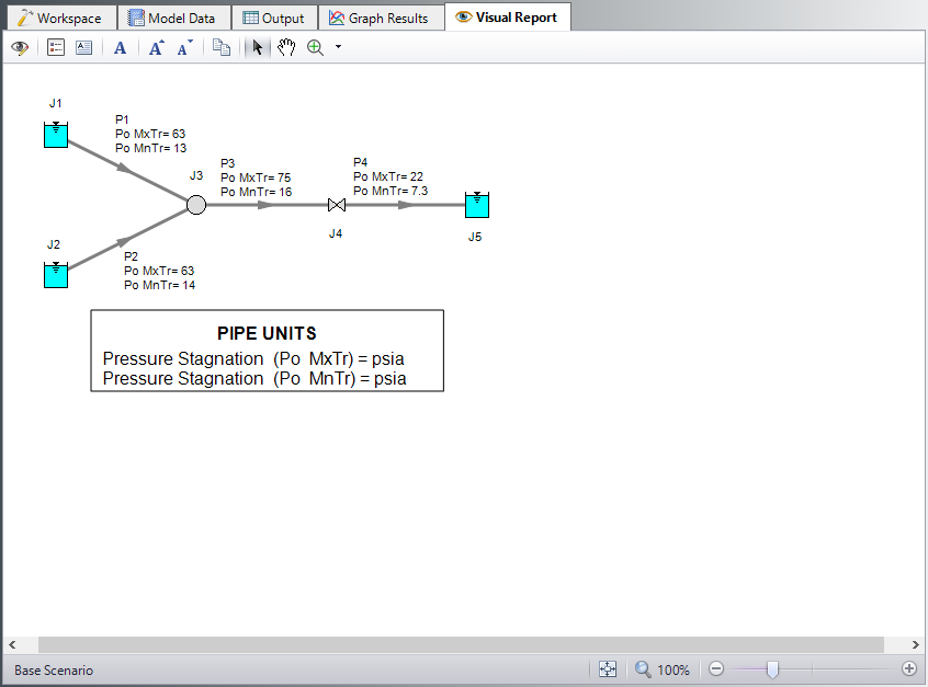
Figure 31: The Visual Report window displays output data on the input schematic. It also can operate in Input Mode where it displays input data
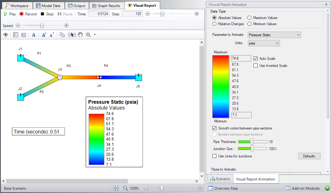
Figure 32: The Visual Report provides an animation feature as an alternate way to view the transient results
Conclusion
You have now used AFT Impulse's five Primary Windows to build and analyze a simple waterhammer model.


