Method of Characteristics
The Method of Characteristics is a general approach for solving a partial differential equation by reducing it to a system of ordinary differential equations.
We see here how it is applied to the transient flow equations. The continuity equation and momentum conservation equation are both partial differential equations. Together, they have two unknowns P and V, and two independent variables x and t. Application of the Method of Characteristics will generate four ordinary differential equations.
Characteristic Equations
The equations are represented below as L1 and L2 .


Linearly combining the equations with the introduction of a constant factor λ


Rearranging terms from the linear combination above

We define a relationship for λ:

Where:

This relationship between wavespeed, time step, and length step must be enforced for this method to work as expected. This is discussed in detail in Pipe Sectioning - Introduction to Method of Characteristics.
Substituting into the above equation:

The terms in the parantheses are simply the total derivatives for P and V.


Simplifying the expression to:

This represents the four characteristic equations that we are searching for, paired as positive (C+) and negative (C-) sets of equations:


Note: There have not been any simplifying assumptions made in the development of these ordinary differential equations - they represent the original partial differential equations exactly.
Numerical Method
We can simplify the equations further into a form that is convenient for simulation.
For the positive characteristic multiply the top equation by a dt, which is equal to dx

Recognizing that sin(α) is simply dz/dx:

It is more convenient to use mass flow instead of velocity, and multiplying through by ρ.

This equation can be integrated along the positive characteristic.
It is useful at this stage to consider a graphical representation of the characteristic grid. Some point P is affected by the positive characteristic from point A, and by the negative characteristic from point B.
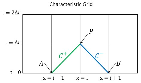
Figure 1: Characteristic grid. The point P sees effects from points A and B after some time dt, which has equal magnitude of dx/a
Setting up the integral, along the positive characteristic line:

Most of the terms are straightforward. However, the third term contains mass flow which varies with respect to x. This term is approximated with the trapezoidal rule, which is second order accurate.

Defining impedance:

and resistance:

and solving for pressure at the point of interest:

we can repeat the above process for the negative characteristic and arrive at:

We have finally arrived a system of two equations with only two unknowns - mass flow and pressure at the point P. These equations can be further arranged into a convenient form known as the compatibility equations.
Related Topics


