Pipe Forces from Valve Closure (English Units)
Valve Closure with Pipe Forces (Metric Units)
Summary
A gravity drain system transfers water from one tank to another through a filter and a valve in the connecting pipeline. It is necessary to determine the transient forces that occur when the valve is partially closed.
Topics Covered
-
Defining force sets
-
Graphing transient forces
-
Evaluating the effect of frictional losses on transient pipe forces
-
Using the isometric pipe drawing mode
-
Generating a CAESAR II force file
Required Knowledge
This example assumes the user has already worked through the Beginner - Valve Closure example, or has a level of knowledge consistent with that topic. You can also watch the Impulse Quick Start Videos, as they cover the majority of the topics discussed in the Valve Closure example.
Model File
This example uses the following file, which is installed in the Examples folder as part of the AFT Impulse installation:
Step 1. Open the Model File
For this example, we will be starting from a pre-built model file which has the fluid, pipes, and junction properties completed to save time.
ØOpen the model file listed above.
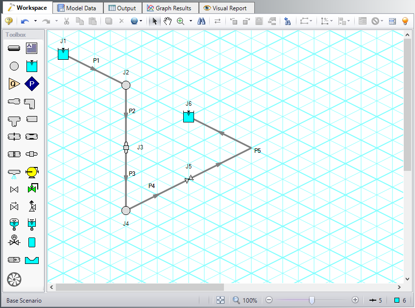
Isometric Pipe Drawing Mode
The previous example models were drawn using the default Pipe Drawing Mode, 2D Freeform. However, AFT Impulse has two additional available drawing modes, 2D Orthogonal and Isometric. Due to the nature of this model the Isometric mode was used to visually interpret the pipe layout and provide a better understanding of the system when analyzing calculated forces.
For future reference when using this feature, the Isometric drawing mode can be turned on in the Arrange menu under Pipe Drawing Mode. It is not recommended to switch the Pipe Drawing Mode once a model has been created and saved. The isometric grid can also be turned on or off from the Arrange menu. When drawing segmented pipes such as P5, a red-dashed preview line will show how the pipe will be drawn on the isometric grid. As you are drawing a pipe, you can change the preview line by clicking any arrow key on your keyboard or scrolling the scroll wheel on your mouse. You can hold the ALT key while adjusting a pipe by the endpoint to add an additional segment. This can be used with the arrow key or mouse scroll wheel to change between different preview line options.
Step 2. Define the Pipe Sectioning and Output Group
ØOpen Analysis Setup and open the Sectioning panel. When the panel is first opened it will automatically search for the best option for one to five sections in the controlling pipe. The results will be displayed in the table at the top. Select the row to use one section in the controlling pipe.
Note: The closer computing stations are to the desired force calculation location, the more accurate the force calculation will be.
Step 3. Define the Transient Control Group
ØOpen the Simulation Mode/Duration panel in the Transient Control group. Enter 10 seconds for the Stop Time.
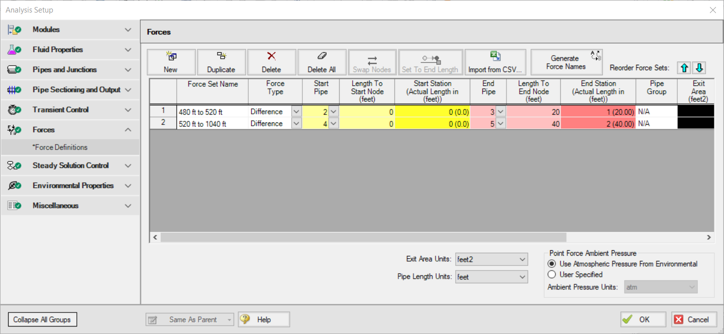
Step 4. Define the Forces Group
ØOpen the Force Definitions panel in the Forces group and define a force set by clicking New, entering the name, the start pipe, length to start node, end pipe, and the length to end node. Repeat this process for the second force set as shown in Figure 3.
A. Force Types
The Difference force type is intended to model the specific case where all of the following criteria is true:
-
The force is between a pair of 90 degree elbows
-
The force is an axial pipe force
-
All pipes, fittings, and components between the elbow pair are in-line
The force equations in the Solver are specific to this geometry. The pipes and components between the elbow pair can be horizontal, vertical, or sloped, but the axial component of the fluid weight is not accounted for in the forces. However, elevation and hydrostatic pressure are accounted for in the pressure and flow solution. Furthermore, AFT Impulse is a hydraulic solver; therefore, only hydraulic forces are calculated. These are forces which act on the pipe from the fluid.
Note: Pipes are assumed to be rigid bodies and AFT Impulse does not account for the effect of pipe deflection on forces.
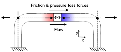
Figure 2: Schematic of the Difference force type
The Point force type would be used for calculating the force at a Dead End junction. It is calculated using the difference in fluid pressure and ambient pressure, multiplied by the pipe area.
The Difference Exit force type would be used between a single 90 degree elbow and a location where the fluid is leaving the system, such as an exit valve, exit orifice, or nozzle.
The force sets in this example will use the Difference force type to calculate the axial forces between 90 degree elbow pairs.
B. Defining Force Sets
Generally it is best to represent each elbow with a unique junction on the Workspace (either an Elbow or Branch). This example assumes that the static pressure loss in the elbows is negligible, and therefore, they are modeled as Branch junctions which are lossless, with exception of the last elbow in Pipe P5 which is visually depicted with a pipe segment. Using explicit junctions on the Workspace will make the Force Definition simple and straightforward, and will also provide an appropriate number of sections. However, this can increase the runtime if the pipes between the elbows have a short length compared to the rest of the pipes in the model. For this reason, Force Sets can also be defined using an intermediate computation station inside a pipe.
The first elbow pair is represented by J2 and J4 which will demonstrate the setup when using explicit junctions. The second elbow pair is represented by J4 and the segment in Pipe P5 which will demonstrate the setup when using an intermidiate station.
Reminder: Segments are simply a visual representation of a bend that can be added to a pipe. They do not represent a pressure loss or elevation change.
ØCreate a force set by clicking New. Then enter the data as shown in Figure 3. Repeat this process for the second force set.
-
Force Set 1:
-
Name =
-
Force Type = Difference
-
Start Pipe = 2
-
Length To Start Node = 0
-
End Pipe = 3
-
Length To End Node =
-
-
Force Set 2:
-
Name =
-
Force Type = Difference
-
Start Pipe = 4
-
Length To Start Node = 0
-
End Pipe = 5
-
Length To End Node =
-
Note: Force sets can also be defined from the Workspace by right-clicking on the starting pipe(s) to automatically create a difference force set from the start node to the end node of that pipe. The force set can then be edited from the Force Definitions panel.
The first force set spans between the first and last computation stations that are between the J2-J4 elbow pair. The start corresponds to the Pipe P2 inlet, therefore, the Start Pipe is P2 and the Length to Start Node is 0
The second force set starts at J4 but ends in the middle of Pipe P5. The start corresponds to the Pipe P4 inlet, therefore, the Start Pipe is P4 and the Length to Start Node is 0
Sectioning has produced one section each in Pipes P2 and P3 for the
In this example, the sectioning conveniently results in computing stations at the locations where we want to calculate forces. Where computing stations do not coincide with the desired force calculation locations, some loss in accuracy will occur. By increasing the number of sections in the controlling pipe during sectioning, a greater number of computing stations will exist, thus reducing the distance to the desired force calculation locations, at the expense of longer run time.
Note: AFT Impulse will set Pipe Station Output automatically to include only those stations required by the force set nodes up to five stations, or all stations if more than five stations are required.
An Impulse model does not contain directional data with regard to the forces, it knows only pipe length and elevation. Since forces are vectors with both magnitude and direction, the user must identify the direction of the calculated forces using data in the pipe arrangement drawing that defines the geometry of the pipe routing. This directional information can then be entered using the Force Unit Vector columns. The force unit vectors will not impact Impulse's calculations, but may be useful if it is desired to export the Impulse force output to a pipe stress software as is discussed later.
ØClick OK to close Analysis Setup.
Step 5. Run the Model
Click Run Model from the Common Toolbar or from the Analysis menu. This will open the Solution Progress window. This window allows you to watch the progress of the Steady-State and Transient Solvers. When complete, click the Graph Results button at the bottom of the Solution Progress window.
Step 6. Graph the Results
ØOn the Quick Access Panel, in the Parameters section, select the Forces tab. The force sets defined on the Force Definitions panel will appear as available forces to graph.
Check the box next to the
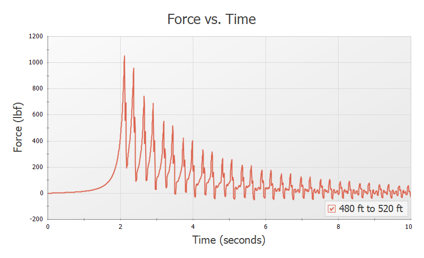
Note that at time zero, which represents the initial, steady-state results, there is no force. This is the expected result for a system at steady-state.
Some traditional methods of analyzing force sets will not have this same result, since they do not include the effects of friction or momentum in their force balances. If the graph from Figure 4 were created with friction and momentum ignored, then the steady-state value would be calculated as approximately
Now create the same graph but for the
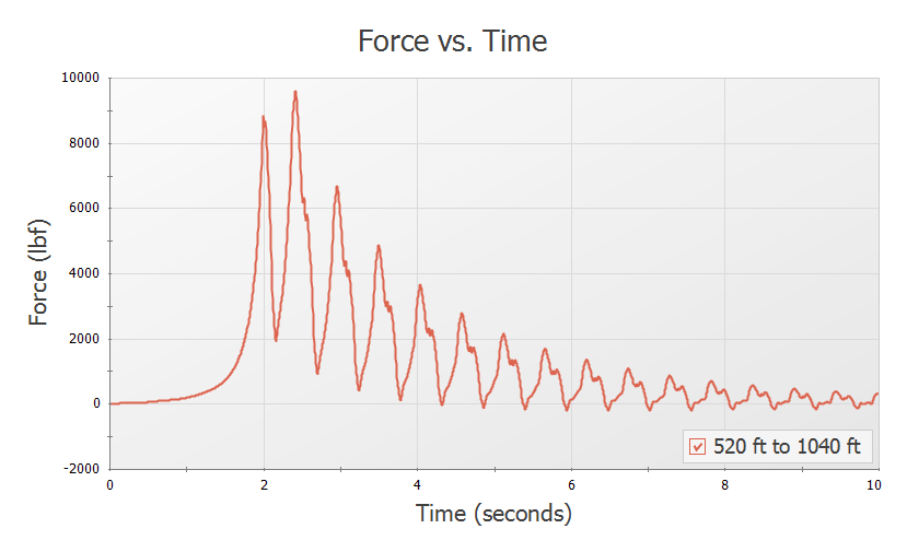
Again we see that with friction included there is no force under steady-state conditions (time zero). If friction were not included, then a steady-state force of approximately
Note: An AFT Impulse model does not contain directional data with regard to the forces, it knows only pipe length and elevation. Since forces are vectors with both magnitude and direction, the user must identify the direction of the calculated forces using data in the pipe arrangement drawing that defines the geometry of the pipe routing.
In summary, there are several important points to be observed:
-
AFT Impulse calculates transient, or time-varying hydraulic forces. This does not include constant loads from fluid, piping, and component weight. A comprehensive analysis of pipe loading must separately include these items.
-
The Difference force type calculates the axial pipe force between a pair of 90 degree elbows.
-
In some cases, ignoring friction and momentum force balance components will result in forces that do not exist in reality, since the frictional forces on the pipe exactly counterbalance the force calculated from the pressure differential at the selected locations.
Step 7. Export CAESAR II Force File
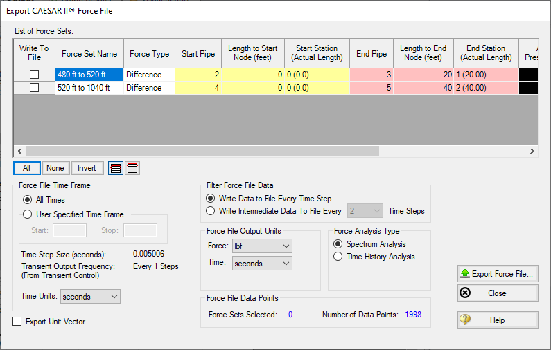
ØGo to the Output window, click on the File menu and select Export Force File and choose CAESAR II Force File, which will open the Export Force File window shown in Figure 6.
The force sets to include in the force file may be individually selected, and all or only intermediate data points may be included in the force file. For the force sets and options selected the number of data points that will be in the file is displayed. This number should not exceed the maximum number of data points allowed in CAESAR II.
In addition, if unit vector information has been entered for the force sets in the Force Definitions panel, the Export Unit Vector option can be used to include this information in the exported file.
Final Note on Transient Cavitation
If transient cavitation occurs, the warning shown in Figure 7 will be displayed in the Output window:
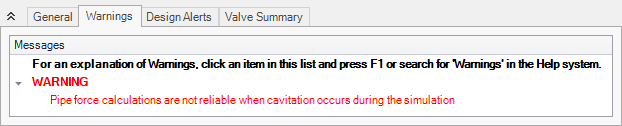
Calculating time varying forces requires a greater level of accuracy in the magnitude and location of pressures, velocity, and frictional losses than may be determined with transient cavitation modeling. Accordingly, pipe force calculations will have a usually indeterminable reduction in accuracy when cavitation occurs.


