Tee/Wye Loss Model
Note: The Detailed tee loss model correlations were developed for steady-state applications. Generally it is not recommended to use the Detailed loss model during the transient run due to increased complexity/runtime, potential instability caused by flow reversal or oscillations, or Artificial Transients. For additional information see the Tee/Wye Waterhammer Theory help topic.
The Simple loss model assumes there are no losses across the tee/wye. The Detailed loss model uses various correlations and data to calculate the loss coefficients across the different flow paths of the tee/wye. Generally, the correlations depend on the flow split, ratio of pipe cross-sectional areas, and angle of the connecting pipes.
-
Sharp Tee - This option represents tees with sharp corners (r/d=0) that have equal areas in the header and an equal or smaller area in the branch (Ac =< Aa = Ab).
-
Rounded Tee - This option represents tees with rounded or smooth corners (r/d=0.1) that have equal areas in the header and an equal or smaller area in the branch (Ac =< Aa = Ab).
-
Area Change Tee - This option represents tees with sharp corners (r/d=0) which have an area sum (Aa + Ac = Ab).
-
Symmetrical Wye - This option represents symmetrical wyes with sharp corners (r/d=0) which have an area sum (Aa + Ab = Ac).
If the cross-sectional area requirements are violated, then the software will still provide results because it accounts for different basis areas and effectively "corrects" the loss coefficient by using velocity ratios. However, it is important to note that in these cases the correlations are still being used outside of their original ranges, so there is inherently some additional uncertainty.
Nomenclature
The correlations and data used by the Detailed loss model come from two different sources: Idelchik's Handbook of Hydraulic Resistance and Miller's Internal Flow Systems (see References below). Each source has their own naming conventions and nomenclature. Furthermore, both nomenclatures assume that the user knows the flow directions ahead of time. For these reasons, AFT has selected a more general nomenclature to describe the names of each pipe in the tee/wye. AFT's nomenclature also accounts for the fact that the user may not know the flow directions ahead of time, and might not be able to properly specify the tee using Idelchik's or Miller's conventions. Since most of the correlations come from Idelchik, and many of our users are familiar with the Idelchik text, we will first describe some of the important nomenclature here. Then, the AFT nomenclature will be depicted below. For reference, Idelchik uses several unusual parameter names; the greek letter Zeta represents the loss coefficient (K factor), "F" represents the cross-sectional area of the pipe, and "w" represents the velocity.
Figure 1 depicts the Idelchik nomenclature, but using "A" for area instead of "F". The pipes are labeled as combined flow (c), straight-through flow (st), and side branch (s). The combined flow pipe always carries the total flow, and depends on if the tee has a diverging or converging flow pattern (flow patterns discussed further in the next section). Loss coefficient subscripts refer to a basis area and location in the tee. For example, Kc,s represents the K factor for the side branch (s) referenced to the combined (c) pipe flow area and velocity. An issue with applying the Idelchik convention to a general software is that sometimes the flow directions are not known ahead of time, or may change based on multiple operational configurations, transient events, etc.
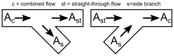
Figure 1: Idelchik’s nomenclature for diverging (left) and converging (right) flow through a Tee/Wye junction
Figure 2 depicts the AFT nomenclature. The pipes are labeled as a, b, and c. The c pipe is always the branching pipe (equivalent to the "s" pipe in Idelchik). This convention allows AFT to cover all flow pattern possibilities discussed below and listed in Table 1 without specifying exactly which pipe is the combined flow pipe.
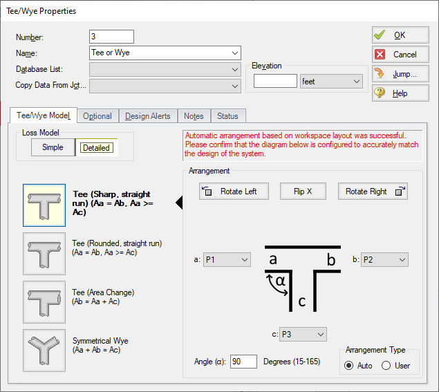
Figure 2: AFT's nomenclature in the Tee/Wye Properties window where the c pipe is always the branch pipe
Flow Patterns & Correlation Selection
There are four general types of flow patterns in tees which depend on the directions of the flow streams:
-
Diverging From Header - flow comes from a single upstream pipe in the header, and a portion of flow diverges into the branch pipe while the remaining portion continues in the straight run.
-
Converging Into Header - flow comes from two upstream pipes, one of which is the header and other is the branch pipe, and the two streams converge into the downstream portion of the header.
-
Dividing From Branch - flow from the branch pipe divides in opposite directions in the header.
-
Combining Into Branch - flow comes from opposite directions in the header and combines into the branch pipe.
The Solver will automatically determine which flow pattern is applicable based on the actual flow directions in the model. The Diverging and Converging patterns use equations or tabulated data with interpolation that come from Idelchik. The Dividing and Combining patterns use tabulated data with interpolation that comes from Miller.
Angle
If the tee angle is 90 degrees, it is not important which pipe you call the a pipe and which the b pipe. The distinction between a and b takes on more importance for non-90 degree pipes. AFT will always define the angle from the a pipe to the c pipe. The user should define the angle according to this definition and be consistent with their physical layout of the pipes. If the actual flow directions in the final solution are different, then the Solver will automatically handle this in the backend.
Some Idelchik correlations are for specific, discreet angles. If the user-entered angle is between these values, then the software will interpolate. Other Idelchik correlations provide equations with the angle as an input, and are valid for a specified angle range. If the angle falls outside of the range, then it will be treated as either the maximum or minimum angle.
The data referenced from Miller was only for 90 degree tees, and therefore, the angle has no effect and is always assumed to be equal to 90 degrees for the Dividing From Branch and Combining Into Branch flow patterns.
Convergence Issues
Sometimes intermediate iterations of the Solver cause a different flow pattern to be selected, and sometimes the system may experience instability as the Solver gets stuck switching back and forth between two different flow patterns. Other times, having many Detailed tees in a pipe network can cause numerical complexity due to the effects of the tees coupling together in such a way that the Solver cannot converge on all of the flow splits. The tee loss coefficients are dependent on the flow splits, but the flow splits are dependent on the other losses in the system. Therefore, if a pipe network contains many tees using the Detailed loss model, when one tee's loss coefficient is updated from an intermediate Solver iteration, the entire network needs to be re-calculated to determine how the flow splits changed. Sometimes this process is not able to terminate within the Tolerances specified by the model.
See the Tee/Wye Junction Complexity help topic for more information and suggestions. In general, if the losses from the tees are small in comparison to the total system losses, or other components that contribute significant pressure loss, then it may be acceptable to assume the tee is lossless and use the Simple loss model.
Negative Loss Coefficients
Under the right conditions it is possible to see a negative loss coefficient for one of the flow paths in the tee. This is physically realistic and is supported in literature by both Idelchik and Miller. In summary, a negative loss coefficient represents an energy/pressure gain for said flow stream of the tee and is achieved by having a portion of kinetic energy transferred to it from the other flow stream. The other flow stream sees an increased loss coefficient (higher than it would have been otherwise), and the net result is still an irrecoverable energy loss across the entire tee control volume. Some specific details are discussed below.
-
Converging Tee Side Branch: Turbulent mixing and momentum exchange takes place between the particles which favors equalization of the velocity field within the pipe which carries the merged flow. In other words, there is a stream with higher energy (velocity/kinetic energy), and a stream with lower energy, and when they merge together they level out to some equilibrium that is somewhere between the high and low energy in the combined flow pipe. The stream which had the higher velocity effectively transfers part of its kinetic energy to the stream with the lower velocity.
-
Evidence from Idelchik 3rd Ed 1994: Diagrams 7-1 to 7-9, the tables and graphs show negative Kc,s values.
-
Evidence from Miller 2nd Ed 1990: Figure 13.10 pg 311, the chart plots lines of constant K factor, some of which have negative values.
-
-
Diverging Tee Straight Run: At certain flow rate ratios (Qs/Qc), a portion of the slowly moving boundary layer adjacent to the wall passes into the side branch while transferring part of the momentum into the straight passage. The increase in energy in the straight passage is associated with a negative Kst, while also accompanied by an increased positive value of Ks such that the whole process is a net irrecoverable pressure loss.
-
Evidence from Idelchik 3rd Ed 1994: Diagrams 7-1 to 7-9, the tables and graphs show negative Kc,st values.
-
Evidence from Miller 2nd Ed 1990: Figure 13.23 pg 319, the curve dips below zero for a range of flow ratios between 0.1 and 0.4.
-
Larger Branching Flows Down a Header
There is an unintuitive, but realistic, situation that can occur due to modeling tees with the Detailed loss model. In some cases, as flow goes down a header pipe past a series of tees, there may be larger flow rates out of the final branching pipes compared to the initial branching pipes (see Figure 3). This is a realistic phenomenon that is caused by the "turning resistance" being larger than the "straight-through resistance"; or in other words, the loss factor for the flow to turn and go out of the branching pipe is larger than the loss factor for the flow to continue straight through the tee. Depending on the boundary conditions and losses in the remaining downstream parts of the network, this may influence the flow to take the path of least resistance and go straight through the tee as opposed to turning and flowing out of the branching pipe.

Figure 3: Illustration of branching flow increasing down the length of a header with a series of Detailed tees
By comparison, a tee modeled as lossless (Simple loss model) has no turning resistance or straight-through resistance. Stagnation pressure decreases continuously down the length of the header due to friction. As a result, the branching flow rates will decrease correspondingly (see Figure 4). The results in Figure 4 with decreasing flow down the header are also possible with the Detailed loss model, and whether you see results more similar to Figure 3 or Figure 4 depend on the pipe network as a whole, including the other losses in the system and the boundary conditions.
 and branching flow decreases down the length of the header")
Figure 4: Illustration of branching flow decreasing down the length of a header (possible with Simple or Detailed loss models)
References
The correlations used by the Detailed loss model are taken mostly from Chapter 7 of Idelchik's Handbook of Hydraulic Resistance (Idelchik 2007)Idelchik, I. E., Handbook of Hydraulic Resistance, 4th edition, Begell House, Redding, CT, 2007., with some additional data taken from Miller's Internal Flow Systems (Miller 1990)Miller, D. S., Internal Flow Systems, 2nd edition, Gulf Publishing Company, Houston, TX, 1990.. Table 1 lists which references are used based on the user's selection in the Tee/Wye Properties window and which flow pattern is applicable as determined by the Solver.
Table 1: References for Tee/Wye junction correlations
| Geometry | Type | Direction | Reference | Page | Diagram / Figure |
|---|---|---|---|---|---|
| Constant Area, Sharp (r/D = 0) | Diverging | Side Branch | Idelchik 2007 | 523 | 7-18 |
| Diverging | Straight Run | Idelchik 2007 | 525 | 7-20 No. 1 | |
| Converging | Side Branch | Idelchik 2007 | 501-504 | 7-1 to 7-4 | |
| Converging | Straight Run | Idelchik 2007 | 501-504 | 7-1 to 7-4 | |
| Dividing | From Branch | Miller 1990 | 323* | 13.27 (r/d=0) | |
| Combining | Into Branch | Miller 1990 | 315* | 13.16 (r/d=0) | |
| Constant Area, Rounded (r/D = 0.1) | Diverging | Side Branch | Idelchik 2007 | 531-533 | 7-23 No. 1 |
| Diverging | Straight Run | Idelchik 2007 | 533 -> 526-527 | 7-23 -> 7-20 No. 1 | |
| Converging | Side Branch | Idelchik 2007 | 511-515 | 7-11 to 7-13 | |
| Converging | Straight Run | Idelchik 2007 | 511-515 | 7-11 to 7-13 | |
| Dividing | From Branch | Miller 1990 | 323* | 13.27 (r/d=0.1) | |
| Combining | Into Branch | Miller 1990 | 315* | 13.27 (r/d=0.1) | |
| Area Sum, Sharp (r/D = 0) | Diverging | Side Branch | Idelchik 2007 | 524 | 7-19 |
| Diverging | Straight Run | Idelchik 2007 | 526-527 | 7-20 No. 2 | |
| Converging | Side Branch | Idelchik 2007 | 505-509 | 7-5 to 7-9 | |
| Converging | Straight Run | Idelchik 2007 | 505-509 | 7-5 to 7-9 | |
| Dividing | From Branch | Miller 1990 | 323* | 13.27 (r/d=0) | |
| Combining | Into Branch | Miller 1990 | 315* | 13.16 (r/d=0) | |
| Wye | Diverging | - | Idelchik 2007 | 545 -> 524 | 7-30 -> 7-19 |
| Converging | - | Idelchik 2007 | 545 | 7-30 | |
|
* Estimates have been made on available data. -> Means the first page number points the reader to a different Diagram. |
|||||


