Wasp-Durand Heterogeneous Slurry Model
(SSL Module Only) The Wasp-Durand Slurry Model is a two-layer slurry approach with heterogeneous (also referred to as the Durand flow) and homogenous fluid components (also referred to as the vehicle component). This method started with the heterogeneous Durand and CondoliosDurand, R., & Condolios, E., "Etude experimentale du refoulement des materieaux en conduites enparticulier des produits de dragage et des schlamms". Deuxiemes Journees de l'Hydraulique, 27-55, 1952. model in the 1950s, was expanded by Wasp et al.Wasp, E. J., Kenny, J. P., & Gandhi, R. L., Solid liquid flow slurry pipeline transportation, Transactions Technical Publications, 1977. in the 1960s and 1970s, and has continued to evolve based on the research of Liu DezhongDezhong, L., Flow Status Identification and Hydraulic Calculation of Tailings Slurry Pipeline, China Minmetals, MCC China ENFI, pp 71-83, No Date., Fei XiangjunXiangjun, Fei, Hydraulics of Slurry and Granular Material Transportation, Tsinghua University Chuxin Society, 1994., Richard W. HanksHanks, R.W. and Dadia, B.H., Theoretical analysis of the turbulent flow of non-newtonian slurries in pipes, AIChE J., 17: 554-557, 1971. [Online]. Available: https://doi.org/10.1002/aic.690170314. and others. This method is used most often with long distance coal pipelines, particularly for coal slurries and slurries with relatively fine particles.
The homogenous component incorporates the viscosity effects of fine particles, similar to the 4-Component Slurry Model, but there is no hard size boundary on which particles can affect the viscosity but finer particles have a greater impact. Similarly, particles of any size may also contribute to the heterogeneous component depending on the degree of stratification for their size group, making Wasp-Durand a model well-suited for finer slurries that may encounter modeling limitations when using Wilson, Addie, Clift or 4-Component slurry models.
Engineering Assumptions
See the SSL Engineering Assumptions topic.
Definition of Solids
Use of Wasp-Durand requires a Granulometric Spread Distribution. This particle size distribution may be defined in either the Solids Library or the Solids Definition Panel of the Analysis Setup Window. A Granulometric Spread Distribution is a histogram-like distribution defined in terms of the fraction of total solids in each size group and the mean particle diameter of each size group.
Stratification in Wasp-Durand is calculated per size group as a ratio of the concentration of solids near the top of the pipe to the concentration of solids towards the middle of the pipe, as shown in Figure 1.
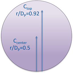
Figure 1: A cross-sectional illustration of the locations within a pipe where Wasp-Durand top and center solids concentrations are defined
Different industries and authors may use different notations for the Wasp-Durand stratification term, but any of the forms shown in Equation 1 are equivalent.
|
|
(1) |

Wasp-Durand is essentially a modular approach, and can be customized using the Wasp-Durand Options area of the Slurry Definition panel.
The deposition velocity is the velocity where solids of a given size have come out of the slurry forming a stationary bed on the bottom of the pipe. For Wasp-Durand, the selection of heterogeneous calculation method determines which method is used for the deposition velocity calculation. The Liu Dezhong deposition velocity calculation is shown in Equations 2 and 3.
|
|
(2) |
|
|
(3) |


Where ρs is the solid density, ρh is the homogenous component density, CV is the volumetric concentration of solids, Vt is the weighted average of sedimentation/terminal velocities of each particle size group in the homogeneous/vehicle fluid, and Vtw is the weighted average of particle sedimentation velocities in a pure carrier fluid (i.e. neglecting viscosity and density effect of fine solids). The m exponent is constant for quasi-homogeneous flow, and variable for more heterogeneous flow regimes.
This version of the Liu Dezhong deposition velocity calculation with the m exponent is from the Chinese national slurry transport code, and differs from the original form in which m is always 6.
Note: The sedimentation velocity terms are calculated using whichever method is specified as the Sedimentation Velocity Model.
The Wasp and Fei Xiangjun equations for deposition velocity are shown in Equations 4 and 5, respectively.
|
|
(4) |
|
|
(5) |


Where ρm is the overall slurry density and fh is the homogeneous Darcy friction factor. Different particle diameters are used by different sources for the Wasp deposition velocity calculation, and we follow Liu Dezhong's convention of using d85.
The sedimentation velocity is per particle size group and is the terminal particle free-fall velocity that occurs when the drag, gravity, and buoyancy forces on a particle are balanced. Both the Ruby & Zanke and Liu Dezhong approaches can be used across a wide range of particle sizes and flow conditions, including laminar, transition, and turbulent flow. Equations 6 and 7 show the Ruby & Zanke (1977) approach for terminal settling velocity.
|
|
(6) |
|
|
(7) |


Where Vt,i is the terminal settling velocity for each particle size group i and μh is the dynamic viscosity of the homogeneous component.
The Liu Dezhong sedimentation velocity calculation is shown in Equations 8-11. The particle size number for each particle size group Nd,i and μf is the clear fluid viscosity. The homogeneous Bingham stiffness factor μph is calculated as shown in Equations 22 and 23.
|
|
(8) |
|
|
(9) |


The weighted average sedimentation velocity is shown in Equation 10. The decimal solid fraction in each band from the Granulometric Spread Distribution is wi.
|
|
(10) |

The total slurry gradient takes the form shown in Equation 11, where i1 is the homogenous gradient and Δi2 is the heterogeneous contribution. The homogeneous gradient will depend on which slurry viscosity model is applied and whether or not Hanks' Bingham plastic is utilized, while the heterogeneous component is calculated with the method specified by the user in the Slurry Definition panel.
|
|
(11) |

The Wasp-Durand heterogeneous gradient is shown in Equations 12-14, where C1V is the volumetric concentration of the homogeneous portion, C2V is the volumetric concentration of the heterogeneous portion, and C1D is the settlement resistance coefficient of particles in the homogenous fluid.
|
|
(12) |
|
|
(13) |
|
|
(14) |


The heterogeneous gradient method for Liu Dezhong in defined in Equations 15 and 16, while Equation 17 defines the Fei Xiangjun approach.
|
|
(15) |
|
|
(16) |
|
|
(17) |


The option to Apply Apparent Slurry Properties allows the viscosity of the homogenous portion to be impacted by the presence of solid particles. These can be Newtonian viscosities, or a non-Newtonian approximation if the Hanks' Bingham Plastic option is enabled. This is described in the next section.
The Newtonian Fei Xiangjun model for apparent viscosity is defined in Equation 18, where CVm is the maximum volumetric concentration.
|
|
(18) |

The Thomas (1965) model for apparent dynamic viscosity of the homogenous component is shown in Equation 19.
|
|
(19) |

The Hanks' Bingham Plastic Approach was developed by Richard W. Hanks. This is a two-layer model that assumes slug or plug flow in an annular distribution, with a constant velocity slug surrounded by a non-Newtonian boundary layer in which frictional losses are concentrated. The general expression for Bingham Plastic shear stress is shown in Equation 20, where τ0 is the yield stress and μph is the effective Bingham stiffness factor of the Wasp-Durand vehicle component.
|
|
(20) |

In the context of the Wasp-Durand approach, Hanks' Bingham Plastic is used to calculate the friction from the vehicle opponent and allows treating this component as apparently non-Newtonian. The yield stress may be user-specified, or calculated using the Fei Xiangjun method in Equation 21.
|
|
(21) |

Where CV0 is the boundary concentration between the Newtonian and non-Newtonian viscosity regimes and CVm is the maximum volumetric concentration. B is an empirical coefficient equal to 8.45 for mineral slurries and 6.87 for coal slurries. The yield stress is a fluid property, and may be calculated in the Analysis Setup Window without running the solver.
Fei Xiangjun also defines a method for calculating the Bingham stiffness factor, shown in Equations 22 and 23, which is used when Fei Xiangjun is selected as the apparent viscosity model and Hanks' Bingham Plastic is enabled in Wasp-Durand options.
|
|
(22) |
|
|
(23) |


The clear fluid friction factor is μf.


