Pump Trip with Check Valve (Metric Units)

Pump Trip with Check Valve (English Units)

Summary

A system pumping water uphill loses power to the pump. A check valve is near the pump discharge. This model predicts the system response and pump speed decay. Uses pump curve and efficiency data.

Topics Covered

• Specifying a pump curve and power curve in the Pump Properties Window

• Using one of the transient pump models which accounts for pump inertia

• Using fittings and losses lumped into a pipe

Required Knowledge

This example assumes the user has already worked through the Beginner - Valve Closure example, or has a level of knowledge consistent with that topic. You can also watch the AFT Impulse Quick Start Video (Metric Units) on the AFT website, as it covers the majority of the topics discussed in the Valve Closure example.

Model File

This example uses the following file, which is installed in the Examples folder as part of the AFT Impulse installation:

• Metric - Pump Trip with Check Valve.fth

Step 1. Start AFT Impulse

From the Start Menu choose the AFT Impulse 10 folder and select AFT Impulse 10.

To ensure that your results are the same as those presented in this documentation, this example should be run using all default AFT Impulse settings, unless you are specifically instructed to do otherwise.

Step 2. Define the Fluid Properties Group

1. Open Analysis Setup from the toolbar or from the Analysis menu.

2. Open the Fluid panel then define the fluid:

   1. Fluid Library = AFT Standard

   2. Fluid = Water (liquid)

      1. After selecting, click Add to Model

   3. Temperature = 21 deg. C

Step 3. Define the Pipes and Junctions Group

At this point, the first two groups are completed in Analysis Setup. The next undefined group is the Pipes and Junctions group. To define this group, the model needs to be assembled with all pipes and junctions fully defined. Click OK to save and exit Analysis Setup then assemble the model as shown in the figure below.

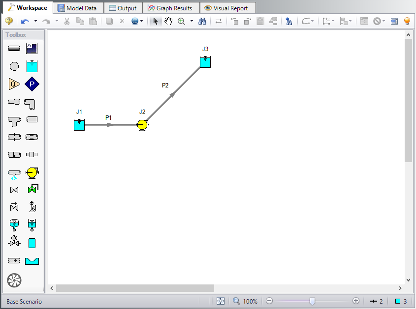
The system is in place but now we need to enter the input data for the pipes and junctions. Double-click each pipe and junction and enter the following data in the properties window.

Junction Properties

1. Reservoir J1

   1. Name = Lower Reservoir

   2. Liquid Surface Elevation = 3 meters

   3. Liquid Surface Pressure = 0 barG (0 kPa(g))

   4. Pipe Depth = 3 meters

2. Pump J2

   1. Inlet Elevation = 0 meters

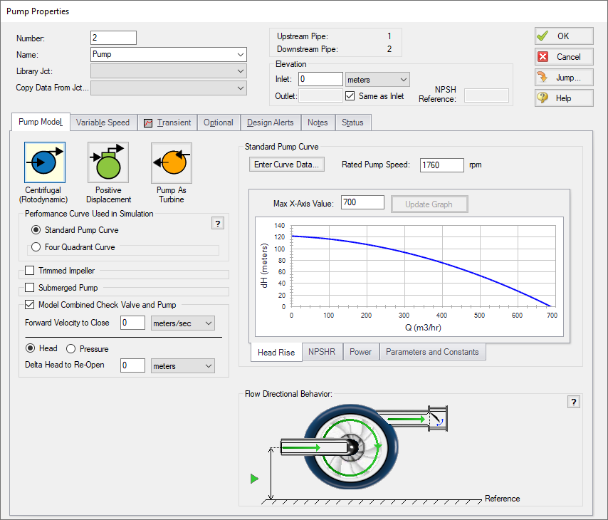
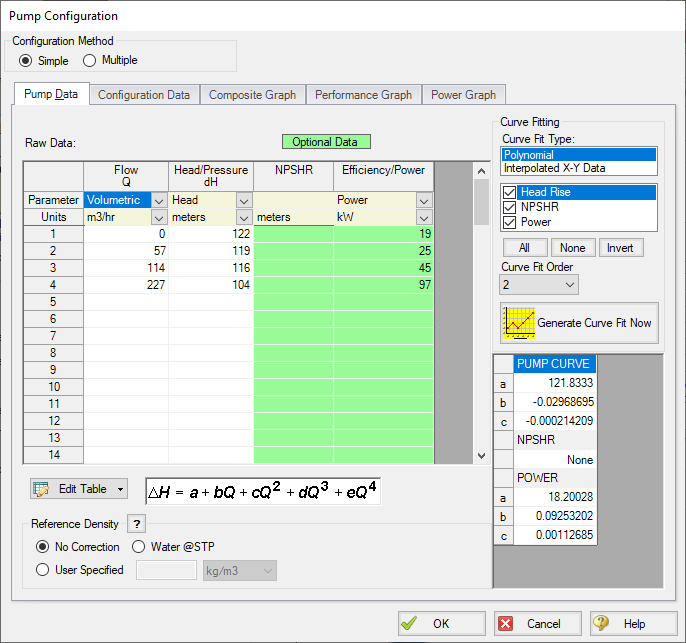
   2. Pump Model tab (Figure 2)

      1. Pump Model = Centrifugal (Rotodynamic)

      2. Performance Curve Used in Simulation = Standard Pump Curve

      3. Model Combined Check Valve and Pump = Checked

      4. Forward Velocity to Close = 0 meters/sec

      5. Delta Head to Re-Open = 0 meters

      6. Rated Pump Speed = 1760 rpm

      7. Enter Curve Data = (Figure 3)

Volumetric	Head	Power
m3/hr	meters	kW
0	122	19
57	119	25
114	116	45
227	104	97

8. Curve Fit Order = 2

3. Transient tab (Figure 4)

   1. Transient = Trip

   2. Transient Special Condition = None

   3. Initiation of Transient = Single Event

   4. Event Type = Time Absolute

   5. Condition = Greater Than or Equal To

   6. Value = 0 seconds

   7. Total Rotating Inertia = User Estimated

   8. Value = 1.05 kg-m2

3. Reservoir J3

   1. Name = Upper Reservoir

   2. Liquid Surface Elevation = 61 meters

   3. Liquid Surface Pressure = 0 barG (0 kPa(g))

   4. Pipe Depth = 3 meters

Pipe Properties

1. Pipe P1

   1. Pipe Material = Steel - ANSI

   2. Size = 4 inch

   3. Type = STD (schedule 40)

   4. Friction Model Data Set = Standard

   5. Lengths = Use table below

Pipe	Length (meters)
1	3
2	302

The pipe model also allows for fittings and losses like valves or elbows. Select the Fittings & Losses tab for P2 and type in 25 for the Total K Factor. Now click OK to close the Pipe Properties window and accept your changes.

Note: Unless specified otherwise, pipe elevation is assumed to vary linearly between junctions. Thus the pipe P2 inlet elevation is 0 meters, and the exit elevation is 58 meters (because the J3 reservoir is 3 meters deep). In between the elevation is linear. If another profile is desired, this can be entered on the pipe’s Optional tab in the Intermediate Pipe Elevations section.

ØTurn on the Show Object Status from the View menu to verify if all data is entered. If there are objects that are not defined, the uncompleted pipes or junctions will have their number shown in red on the workspace. If this happens, go back to the uncompleted pipes or junctions and enter the missing data. If all objects are defined, the Pipes and Junctions group in Analysis Setup will have a check mark.

Step 4. Define the Pipe Sectioning and Output Group

ØOpen Analysis Setup and open the Sectioning panel. When the panel is first opened it will automatically search for the best option for one to five sections in the controlling pipe. The results will be displayed in the table at the top. Select the row to use one section in the controlling pipe. 

Step 5. Define the Transient Control Group

ØOpen the Simulation Mode/Duration panel in the Transient Control group. Enter 30 seconds for the Stop Time.

All groups should now be complete and the model is ready to run. If all groups in Analysis Setup have a green checkmark then Click OK and proceed. Otherwise, enter the missing information.

Step 6. Run the Model

Click Run Model from the toolbar or from the Analysis menu. This will open the Solution Progress window. This window allows you to watch the progress of the Steady-State and Transient Solvers. When complete, click the Output button at the bottom of the Solution Progress window.

Step 7. Examine the Output

The Output window will display any warnings if they exist. There should not be any warnings here. The Graph Results window will be more useful in understanding the results. Go to the Graph Results window.

First, graph the static pressure.

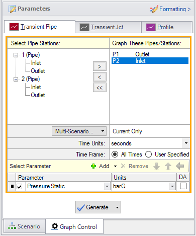
1. On the Quick Access Panel, on the Transient Pipe tab, add the Pipe 1 Outlet and Pipe 2 Inlet (see Figure 5). These represent the pump suction and discharge locations.

2. For Parameter, select the Pressure Static.

3. Set the units to barG.

4. Click Generate.

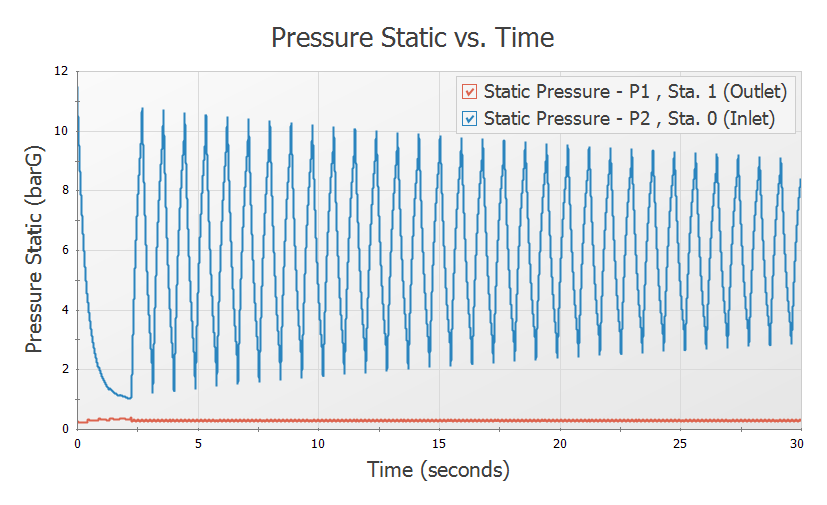
The resulting pressure transients are shown in Figure 6. Here one can see that the transient pressure at the pump discharge does not rise above the initial steady-state pressure. This is not always the case.

Next, graph the pipeline transient pressure profile

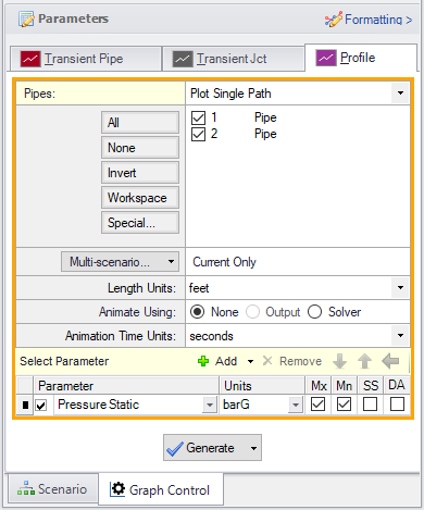
1. On the Quick Access Panel, select the Profile tab (Figure 7).

2. In the Pipes area select All to select both pipes 1 and 2.

3. In the Parameter area make sure Pressure Static is selected.

4. Set the static pressure units to barG.

5. Make sure boxes are checked for Mx and Mn which will plot the maximum and minimum values.

6. Click Generate.

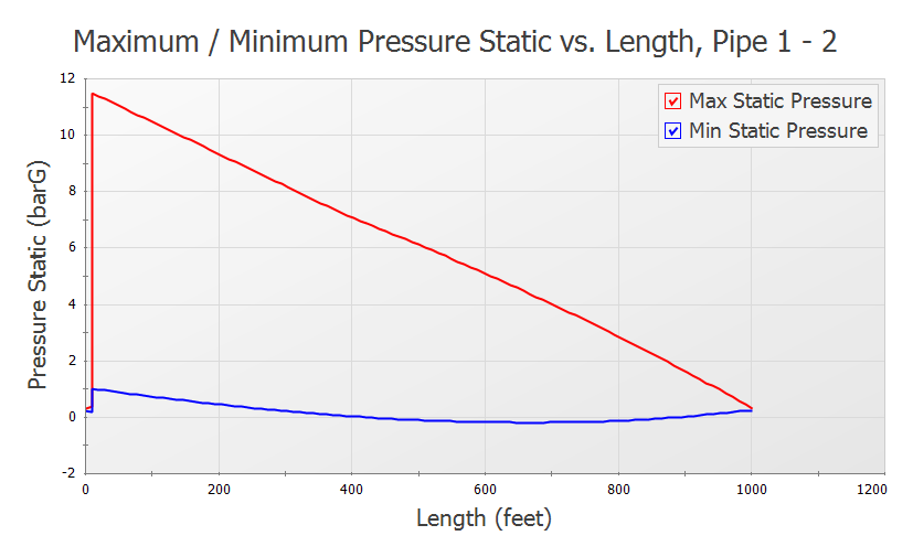
Profile type graphs that show maximum and minimum values can be very helpful. In Figure 8 we see that the maximum transient pressure occurs at the pump discharge, and that the minimum pressure occurs 190-220 meters downstream of the pump. Also note that minimum pressure goes below atmospheric pressure for almost 140 meters of pipe. For some applications this may not be acceptable.

Finally, graph the pump speed decay.

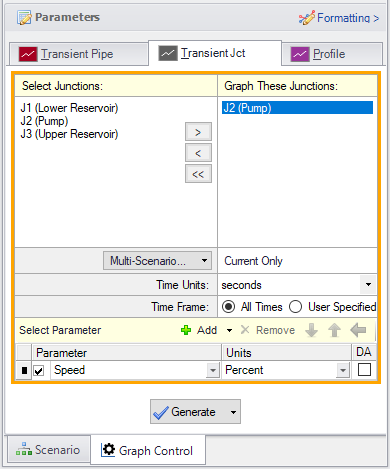
1. Select the Transient Jct tab on Quick Access Panel.

2. Add J2 (Pump) to the Graph These Junctions list on the Transient Jct tab (see Figure 9).

3. For the parameter to graph, make sure Speed is selected.

4. Click Generate.

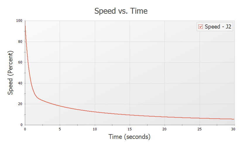
The predicted pump speed is then shown (Figure 10).