Tank Blowdown Example (English Units)
For the Metric units version of this example. click here.
Summary
This
Topics covered
-
Model building basics
-
Entering pipe and junction data
-
Entering transient data
-
Graphing output results
Required knowledge
This example assumes the user has not used AFT xStream previously. It begins with the most basic elements of laying out the pipes and junctions and solving the transient system via the Method of Characteristics (MOC).
Model file
Step 1. Start AFT xStream
-
ØTo start AFT xStream, click Start on the Windows taskbar and open AFT xStream. (This refers to the standard menu items created by setup. You may have chosen to specify a different menu item).
After AFT xStream starts, the Startup window, as shown in Figure 1, appears. This window provides you with several options before you start building a model:
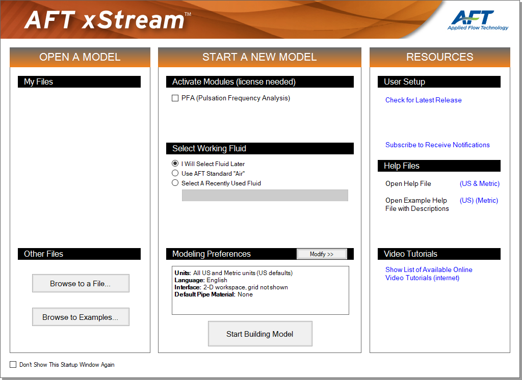
-
Click "Start Building Model".
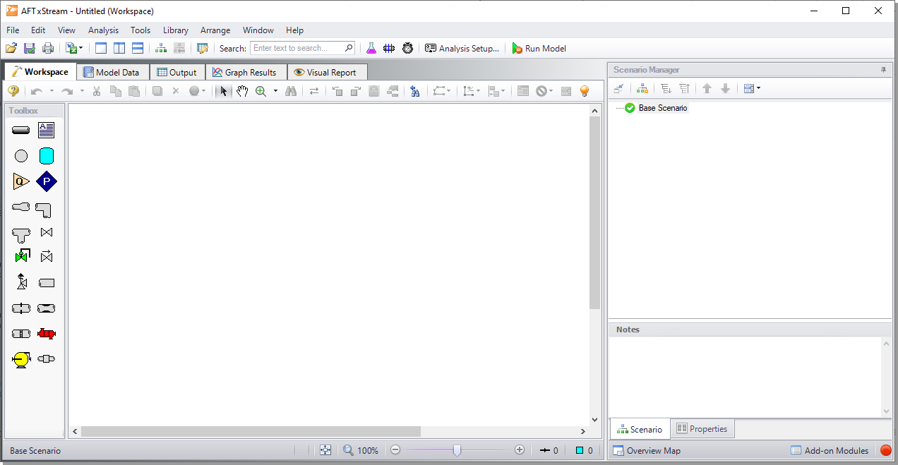
The Workspace window is initially the active window, as seen in Figure 2.
AFT xStream supports dual monitor usage. You can click and drag any of the five primary window tabs off of the main xStream window. Once you drag one of the primary windows off of the xStream window, you can move it anywhere you like on your screen, including onto a second monitor in a dual monitor configuration. To add the primary window back to the main xStream primary tab window bar, simply click the "X" button in the upper right of the primary window.
To ensure that your results are the same as those presented in this documentation, this example should be run using all default AFT xStream settings, unless you are specifically instructed to do otherwise.
The Workspace window
The Workspace window is the primary interface for building your model. This window has three main areas: the Toolbox, the Quick Access Panel, and the Workspace itself. The Toolbox is the bundle of tools on the far left. The Quick Access Panel is displayed on the far right. It is possible to collapse the Quick Access Panel by clicking on the thumbtack pin in the upper right of the Quick Access Panel in order to allow for greater Workspace area. The Workspace takes up the rest of the window.
You will build your pipe flow model on the Workspace using the Toolbox tools. The Pipe Drawing tool, on the upper left, is used to draw new pipes on the Workspace. The Annotation tool allows you to create annotations and auxiliary graphics.
Below the two drawing tools are icons that represent the different types of junctions available in AFT xStream. Junctions are components that connect pipes and also influence the pressure or flow behavior of the pipe system. The junction icons can be dragged from the Toolbox and dropped onto the Workspace.
When you pass your mouse pointer over any of the Toolbox tools, a tooltip identifies the junction's function.
Step 2. Lay out the model
To lay out the tank blowdown model, you will place a Tank junction, a Valve junction, and an Assigned Pressure junction on the Workspace. Then you will connect the junctions with pipes.
I. Place the Tank junction
-
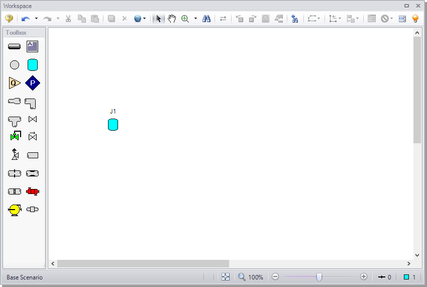
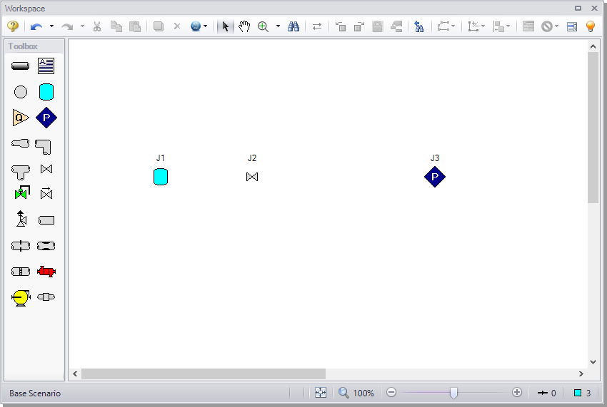
ØTo start, click and drag a Tank junction from the Toolbox and drop it on the Workspace. Figure 3 shows the Workspace with one Tank.
Items placed on the Workspace are called objects. All objects are derived directly or indirectly from the Toolbox. AFT xStream uses three types of objects: pipes, junctions and annotations.
All pipe and junction objects on the Workspace have an associated ID number. For junctions, this number is, by default, placed directly above the junction and prefixed with the letter "J". Pipe ID numbers are prefixed with the letter "P". You can optionally choose to display either or both the ID number and the name of a pipe or junction. You also can drag the ID number/name text to a different location to improve visibility.
The Tank you have created on the Workspace will take on the default ID number of one. You can change this to any desired number greater than zero, but less than 100,000.
Editing on the Workspace
Once on the Workspace, junctions can be moved to new locations and edited using the features on the Edit menu. Cutting, copying, and pasting are all supported. Undo is available for most formatting and arrangement actions on the Workspace.
Note: The relative location of objects in AFT xStream is not important. Distances and heights are defined through dialog boxes. The relative locations on the Workspace establish the connectivity of the objects, but have no bearing on the actual length or elevation relationships.
II. Place the Valve junction
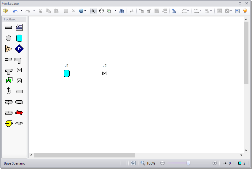
ØTo add a Valve junction, click and drag a valve from the Toolbox and place it on the Workspace as shown in Figure 4. The Valve will be assigned the default number "J2".
III. Place an Assigned Pressure junction
ØTo add an Assigned Pressure junction, click and drag an Assigned Pressure junction from the Toolbox and place it on the Workspace as shown in Figure 5. The Assigned Pressure junction will be assigned the default number "J3".
ØBefore continuing, save the work you have done so far. Choose Save As... from the File menu and enter a file name (Tank Blowdown, perhaps) and AFT xStream will append the ".xtr" extension to the file name.
IV. Draw a pipe between J1 and J2
Now that you have all of the junctions, you need to connect them with pipes.
-
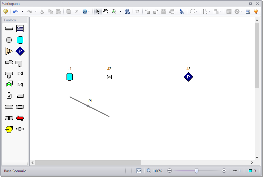
ØTo create a pipe, click the Pipe Drawing Tool icon on the Toolbox. The pointer will change to a crosshair when you move it over the Workspace. Draw a pipe above the junctions by clicking and dragging the mouse, similar to that shown in Figure 6.
The pipe object on the Workspace has an ID number (P1) that is shown near the center of the pipe.
-
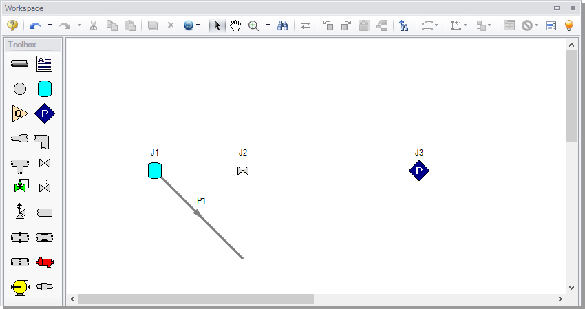
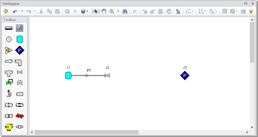
ØTo place the pipe between J1 and J2, use the mouse to grab the pipe in the center and drag it so that the left endpoint falls within the J1 Tank icon, then drop it there (see Figure 7). Next, grab the right endpoint of the pipe and stretch the pipe, dragging it until the endpoint terminates within the J2 Valve icon (see Figure 8).
Reference positive flow direction
Located on the pipe is an arrow that indicates the reference positive flow direction for the pipe. AFT xStream assigns a flow direction corresponding to the direction in which the pipe is drawn. You can reverse the reference positive flow direction by choosing Reverse Direction from the Arrange menu or selecting the Reverse Pipe Direction button on the Workspace Toolbar.
The reference positive flow direction indicates which direction is considered positive. If the reference positive direction is the opposite of that obtained by the Solver, the output will show the flow rate as a negative number.
V. Add the remaining pipe
A faster way to add a pipe is to draw it directly between the desired junctions.
-
ØActivate the Pipe Drawing Tool again. Position the cursor on the J2 Valve, then press and hold the left mouse button. Stretch the pipe across to the J3 Assigned Pressure junction, then release the mouse button. All objects in the model should now be graphically connected as they are in Figure 9.
Save the model by selecting "Save" in the File menu, by clicking the "Save" icon on the Toolbar, or by entering Ctrl+S.
Note: It is generally desirable to lock your objects to the Workspace once they have been placed. This prevents accidental movement and disruption of the connections. Locking also helps prevent accidental deletion of your output once a solution has been completed. You can lock all the objects by choosing Select All from the Edit menu, then selecting Lock Object from the Arrange menu. The Lock Object button on the Workspace Toolbar will appear depressed indicating it is in an enabled state, and will remain so as long as any selected object is locked.

A. Define the model components
Object status
Each pipe and junction has an object status. The object status tells you whether the object is defined according to AFT xStream's requirements. To see the status of the objects in your model, click the light bulb icon on the Workspace Toolbar (alternatively, you could choose "Show Object Status" from the View menu). Each time you click the light bulb, "Show Object Status" is toggled on or off.
When "Show Object Status" is on, the ID numbers for all undefined pipes and junctions are displayed in red on the Workspace. Objects that are completely defined have their ID numbers displayed in black. (These colors are configurable through User Options from the Tools menu.)
Because you have not yet defined the pipes and junctions in this model, all the objects' ID numbers will change to red when you turn on "Show Object Status."
Another useful feature is the List Undefined Objects window (Figure 10). This can be opened from the View menu by clicking on "List Undefined Objects", or by clicking the List Undefined Objects icon on the Workspace toolbar . All objects with incomplete information are listed. Click on an undefined pipe or junction to display the property data that is missing. Click the close button on the bottom right to stop showing this window.
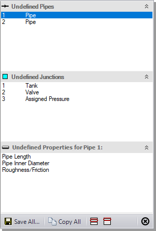
Figure 10: The List Undefined Objects window lets you see the undefined properties for each undefined object
I. Enter data for Tank
As shown in Figure 9, the J1 junction is a Tank junction.
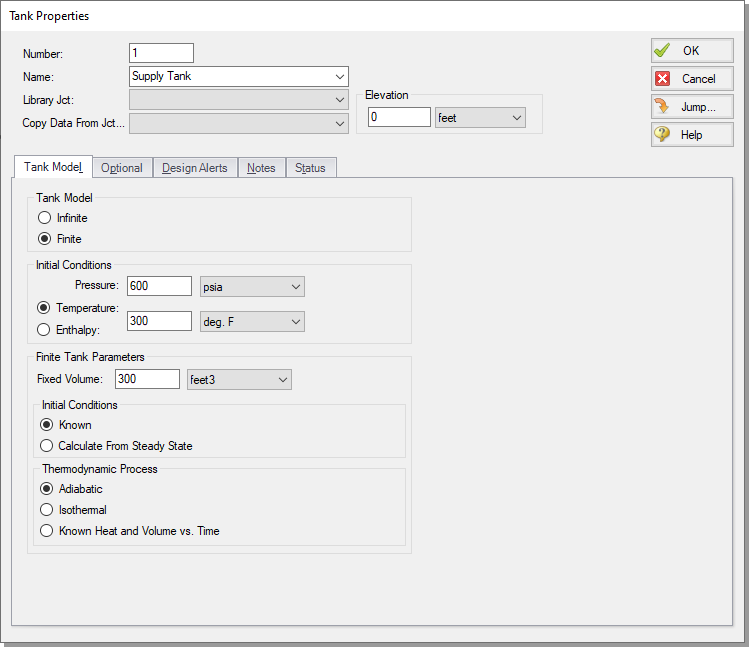
ØTo define the first tank, open the J1 Tank Properties window (See Figure 11) by double-clicking on the J1 icon.
Note: You can also open an object's Properties window by selecting the object (clicking on it) and then either pressing the Enter key or clicking the Open Pipe/Junction Window icon on the Workspace Toolbar.
ØEnter a Pressure of
Note: You can specify default units for many parameters (such as
By default, the junction's name is the junction type. The name can be updated by entering it in the Name field at the top of the window. In Figure 11, the name of Tank J1 is "Supply Tank." The name can be displayed on the Workspace, Visual Report, or in the Output.
Most junction types can be entered into a custom Junction Library allowing the junction to be used multiple times or shared between users. To select a junction from the custom library, choose the desired junction from the Library List in the junction's Properties window. The current junction will get the properties from the library component.
The "Copy Data From Jct..." list will show all the junctions of the same type in the model. This will copy desired parameters from an existing junction in the model to the current junction.
The Tank Model tab is the tab that appears first when the Tank junction is opened and contains all of the inputs required to define the Tank in steady-state. While the Tank Model tab is specific to the Tank junction, the first tab opened for any junction will contain all inputs required for that junction to be defined.
The Optional tab allows you to enter different types of optional data. You can select whether the junction number, name, or both are displayed on the Workspace. Some junction types also allow you to provide a guess for initial pressure as well as other junction specific data.
Each junction has a tab for notes, allowing you to enter text describing the junction or documenting any assumptions.
The highlight feature displays all the required information in the Properties window in light blue. The highlight feature is on by default. You can toggle the highlight off and on by double-clicking anywhere in the window or by pressing the F2 key. The highlight feature can also be turned on or off in the User Options window, or accessed from the View menu by selecting the "Highlight in Pipe and Jct Windows" option.
The Status tab will state whether all required input data is present for a given junction. If not, it will list all inputs that are incomplete.
-
ØClick OK. If "Show Object Status" is turned on, you should see the J1 ID number turn black again, telling you that J1 is now completely defined.
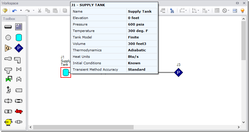
You can check the input parameters for J1 quickly, in read-only fashion, by using the Inspection feature. Position the cursor on the Tank J1 junction and hold down the right mouse button. An information box appears, as shown in Figure 12.
Inspecting is a faster way of examining the input (and output, if output results are available) than opening the Properties window.
II.
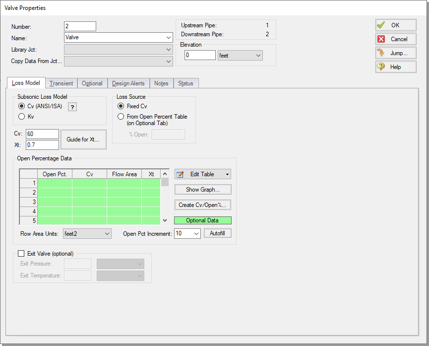
ØOpen the J2 Valve Properties window (see Figure 13) and enter an elevation of 0
ØChoose the loss model as
ØClick on the Optional tab and, under Special Condition, select Closed. This indicates the valve will be closed in the steady state.
ØClick the Transient tab and enter the data below for
| Time (seconds) | Cv | Xt |
|---|---|---|
| 0 | 0 | 0.7 |
| 0.1 | 60 | 0.7 |
| 240 | 60 | 0.7 |
The first data point (
Note: The initial transient data point is
The J2 Valve is the element which causes the transient in this model. The purpose of the model will be to understand how the conditions within the supply tank and discharge pipe change after the valve opens.
When transient data is entered for a junction, an "XT" symbol is shown next to the junction number on the Workspace.
III.
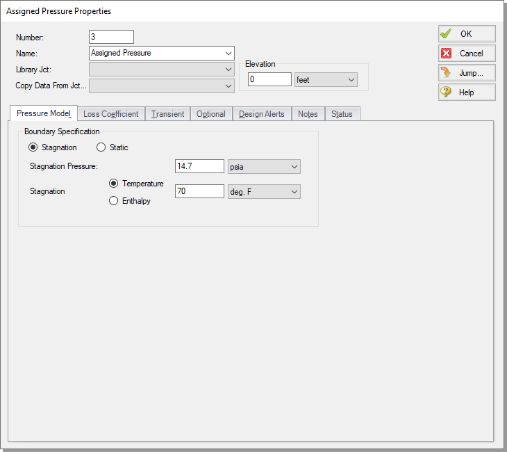
ØOpen the J3 Assigned Pressure Properties window (see Figure 15) and enter an Elevation of 0
ØEnter a Stagnation Pressure of
ØSave the model again before proceeding.
IV.
The next step is to define all the pipes. Double-click the pipe object on the Workspace.
-
ØFirst, open the Pipe Properties window for Pipe P1.

The Pipe Properties window offers control over all important flow system parameters that are related to pipes.
The Inspect feature also works within the Pipe Properties window. To inspect a connected junction, position the mouse pointer on the connected junction's ID number and hold down the right mouse button. This is helpful when you want to quickly check the properties of connecting objects. (You can also use this feature in junction Properties windows for checking connected pipe properties.)
By double-clicking the connected junction number, you can jump directly to the junction's Properties window, or you can click the Jump button to jump to any other part of your model.
Click OK to finish defining P1.
V.
ØOpen the Pipe Properties window for Pipe P2. Enter a length of
Check if all the pipes and junctions are defined by clicking on the List Undefined Objects button. If all data is entered, no items should appear in the Undefined Objects window. If items are present, open the corresponding Properties windows for the incomplete items from the workspace. The Status tab on each Properties window will indicate what information is missing.
B. Review model data
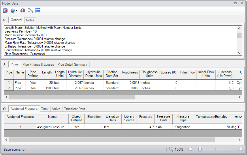
ØSave the model. It is also a good idea to review the input using the Model Data window.
Reviewing input in the Model Data window
The Model Data window is shown in Figure 17. To change to this window, you can select it from the Window menu, you can click on the Model Data tab, or you can press Ctrl+M. The Model Data window gives you a text based perspective of your model. Selections can be copied to the clipboard and transferred into other Windows programs, exported into Excel, saved to a formatted file, printed to an Adobe™ PDF, or printed out for review.
Data is displayed in three general areas. The top is called the General data section, the middle is the Pipe data section and the bottom is the Junction data section. Each section is collapsible using the button at the top left of the section. Further, each section can be resized.
The Model Data window allows access to all Properties windows by double-clicking on any input parameter column in the row of the pipe or junction you want to access.
Step 3. Specify Analysis Setup
-
ØNext, click Analysis Setup on the Main Toolbar to open the Analysis Setup window (see Figure 19). The Analysis Setup window contains six or more groups depending on which modules you may be using. Each group has one or more items. A fully defined group has every item within it defined with all required inputs. Complete every group to run the Solver. A group or item that needs more information will have a red exclamation point to the left of the group or item name. After completing a group, the group icon shows a green circle with a checkmark. After defining all groups, thus completing the Analysis Setup, the Model Status light in the lower right corner of the Workspace turns from red to green.
The Analysis Setup window can also be opened by clicking on the Model Status Light on the Status Bar at the bottom right corner of the AFT xStream window.
A. Specify the Modules group
Under the Modules group, click on the Modules item to open the Modules panel, shown in Figure 19. Here you can enable and disable the Pulsation Frequency Analysis add-on module. By default, the model will have all modules disabled. Therefore, make no changes to this panel for this example.
B. Specify the Fluid Properties group
-
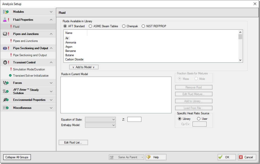
ØSelect the Fluid item to open the Fluid panel (Figure 20).
This panel allows you to specify the fluid used in the model.
You can select a fluid from the standard AFT xStream fluid library (AFT Standard), or select ASME Steam Tables. Additionally, you can select multiple fluids and/or create mixtures using the included NIST REFPROP library or optional add-on Chempak library
-
ØSelect the AFT Standard fluid option, then choose "Nitrogen (GN2)" from the list and click the "Add to Model" button.

C. Inspect the Pipes and Junctions group
The Pipes and Junctions group in the Analysis Setup window contains the Pipes and Junctions panel, which is used to show the status of the pipes and junctions on the workspace. This item is incomplete if there are any undefined pipes/junctions on the Workspace, or if there are no pipes/junctions on the Workspace. In this example the objects in the Workspace are fully defined, so this item is marked as complete.
Running models in steady-state
After fully specifying the pipes and junctions, sufficient information exists to run the model in steady-state. You can run the model in steady-state by selecting the Simulation Mode/Duration panel from the Transient Control group and then choosing "AFT Arrow™ Steady" for the Time Simulation. If you do this, the other inputs on the Simulation Mode/Duration panel and the Pipe Sectioning and Output panel will no longer be required, and the model can be run.
In general, it is a good idea to always run your model in steady-state before running the full transient analysis to make sure the model is giving reasonable results. However, in this case the model has no flow in the steady state, and a steady state run is trivial.
D. Specify the Pipe Sectioning and Output group
The next panel is the Pipe Sectioning and Output panel in the corresponding group. The Pipe Sectioning and Output panel divides pipes into computation sections in a manner which is consistent with the Method of Characteristics (MOC).
To satisfy the MOC, the following equation must be satisfied:

where Δt is the time step, Δx is the section length, and c is the sonic velocity.
-
ØEnter "1" for the Minimum Number of Sections Per Pipe
The Minimum Number of Sections Per Pipe determines the section length by taking the quotient of the shortest pipe's length and the Minimum Number of Sections.
-
ØDefine the Estimated Maximum Pipe Temperature During Transient as
The Estimated Maximum Pipe Temperature During Transient is used to calculate the maximum sonic velocity. Since all pipes in the network must be solved together, the time step must be the same for each pipe. However, the sonic velocity will not be equivalent for all of the pipes. Therefore, the sonic velocity at the specified maximum temperature is used to find a uniform time step for the system. Without a uniform time step, the MOC could fail. Choosing a maximum temperature that is much higher or much lower than the maximum temperature calculated during the run can result in additional uncertainty in the MOC solution
The Sectioning Summary underneath the inputs will be partially filled in. Certain properties, such as total steps and total pipe computations, need the Simulation Mode/Duration panel completed to be defined.
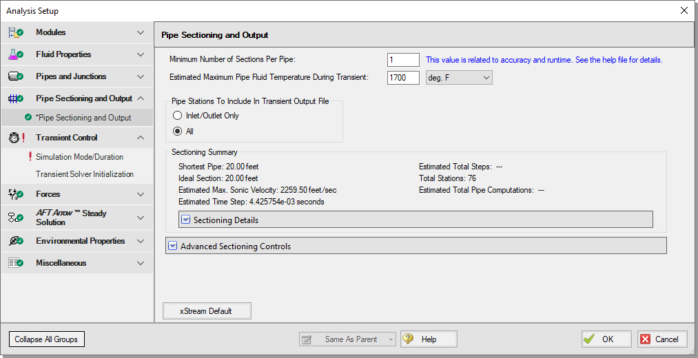
Figure 21: The Sectioning panel in the Analysis Setup window is used to calculate the time step of the model
E. Specify the Transient Control group
The Transient Control group has two items, the Simulation Mode/Duration panel and the Transient Solver Initialization panel. The Simulation Mode/Duration panel allows you to choose the simulation type, and to specify the time that the simulation starts and stops.
The Transient Solver Initialization panel contains advanced settings related to the resolving artificial transients in the model, and typically should not be changed.
-
ØSelect the Simulation Mode/Duration panel (Figure 22). Enter 0 seconds for Start Time and 240 for Stop Time.
-
ØClick OK to accept the current settings. The last Analysis Setup panel should be completed. The model is ready to be solved.

Figure 22: The Simulation Mode/Duration panel is used to specify the simulation type and the time span for the transient
-
ØSave the model.
Step 4. Run the solver
-
ØChoose "Run Model..."from the Analysis menu or click the "Run Model" button on the Main Toolbar. During execution, the Solution Progress window displays the state of the simulation (Figure 24). You can use this window to pause or cancel the solver's activity.
Note the run time may take 5-10 minutes for this model, depending on your computer's speed.
The two solvers
AFT xStream has two solvers. The first is called the AFT Arrow™ Steady Solver, which as its name suggests, obtains a steady-state solution to the pipe network. The second solver is called the Transient Solver and solves the gas transient equations.
The AFT Arrow™ Steady solver and Transient solver use different sectioning methods, which causes small discrepancies between the converged AFT Arrow™ Steady solution and the first time step of the transient solution. To allow artificial waves caused by these discrepancies to die out, AFT xStream runs the Transient solver for a period of time before the transient simulation begins. Once the artificial transients have died out AFT xStream checks the solution with resolved artificial transients against the AFT Arrow™ Steady solution. If the mismatch between the beginning and end of the artificial transient resolution process is sufficiently small AFT xStream proceeds with the transient simulation. See the chart in Figure 23 as a visual representation of the process described above.
![]()
Figure 23: Illustration of the Transient Solver Initialization process with artificial transient resolution
ØWhen the solution is obtained, click the Output button to display the text-based Output window. The information in the Output window can be reviewed visually on the screen, saved to a file, exported to a spreadsheet-ready format, copied to the clipboard, or printed.

When the Transient Solver runs, the transient output data is written to a file. This file is given the same name as the model itself with a number appended to the name, and with an ".out" extension appended to the end. For all transient data processing, graphing, etc., the data is extracted from this file. The number is appended because AFT xStream allows the user to build different scenarios all within this model. Each scenario will have its own output file; therefore, the files need to be distinguishable from each other.
The output file will remain on disk until the user erases it or the model input is modified. This means that if you were to close your model right now and then reopen it, you could proceed directly to the output window for data review without re-running your model.
Step 5. Review the Output window
Click Output after the solver is finished. The Output window (Figure 25) is similar in structure to the Model Data window. Three areas are shown, and you can minimize or enlarge each section by clicking the arrow next to the General, Pipes, and All Junctions tabs. The items displayed in the tabs can be customized with the Output Control window from the Tools drop-down menu.
The General section will open by default to the Warnings tab if any Warnings or Cautions were encountered during the simulation. This model should generate a Caution that the Maximum Transient Pipe Mach Number is at least 0.2 higher than the steady pipe Mach number, which occurs since there is no flow in the system at steady state. When this Caution is present, the effect of pipe sectioning on results can be significant. The impact of pipe sectioning will be addressed in greater detail later in Step 10.
The Output window allows you to review both the steady-state and transient results. The Pipes tab, All Junctions tab, and any specific junction tabs in the Junction section (such as Branch, Tank, Valve, etc.) show the steady-state results.
Click on the Event Messages By Time tab (See Figure 28). There should be messages indicating that Valve J2 experienced a near instantaneous choking that dissipated after about 0.06 seconds while Assigned Pressure J3 experienced choking after 2.
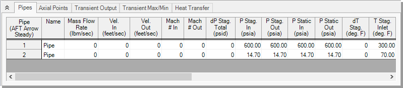
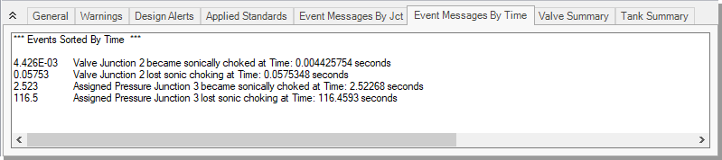
Figure 28: The Output window displays event messages about system behavior in the Event Messages by Time tab
A. Modify the output format
Go to the Transient Max/Min tab in the Output window. If you selected the default AFT xStream Output Control, the Max. Mass Flowrate and Min. Mass Flowrate should have units of
ØSelect Output Control from the Tools menu or the main Toolbar. Open the Pipe Transient results section. On the right side of the Pipe Transient results section is the list of currently selected output parameters (see Figure 29). Click and change the units by clicking the arrow beside the units, and then selecting
ØClick OK to display changes to the current results. You should see both the Max. Mass Flowrate and Min. Mass Flowrate in units of
Ø Select Output Control from the Tools menu one more time. Open the Transients Results section. The Reorder scroll bar on the far right allows you to reorder parameters in the list. You may also reorder parameters by dragging and dropping the icon just to the left of each parameter within the list of currently selected parameters.
ØSelect the Temperature Static parameter and use the Reorder scroll bar to move it up to the top of the parameter list.
ØClick OK to display the changes to the current results. You will see in the Transient Max/Min table that the first column now contains Temperature Static. The Output Control window allows you to obtain the parameters, units and order you prefer in your output. This flexibility will help you work with AFT xStream in the way that is most meaningful to you, reducing the possibility of errors.
ØLastly, double-click the column header Max. Mass Flowrate in the Transient Max/Min tab. This will open a window in which you can change the units once again if you prefer. These changes are extended to the Output Control parameter data you have previously set.
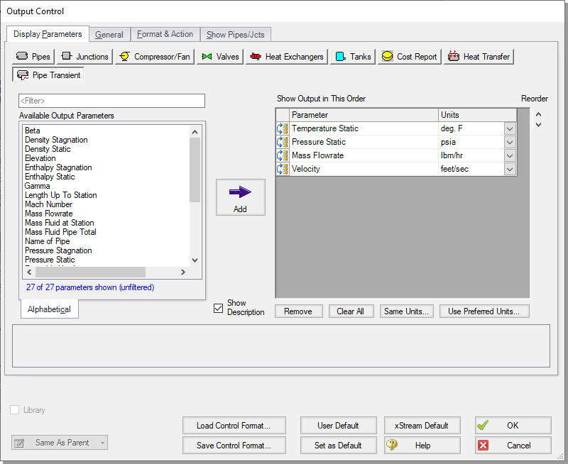
Figure 29: The Output Control window allows for the modification of Parameters shown, Units, and the Order of Results
B. Graph the results
For transient analysis, the Graph Results window will usually be more helpful than the Output window because of the more voluminous data.
-
ØOpen the Graph Results window by choosing it from the Windows menu, clicking the Graph Results tab, by clicking "Graph Results" from the Solution Progress window after running the model, or by pressing Ctrl+G.
 (Add button) the outlet station. This pipe computing station correlates to the pipe discharge for the Blowdown Tank system. Select the Graph Parameter as Temperature Static and set the units to
![]()
Figure 30: The Graph Control tab on the Quick Access Panel allows you to specify the graph parameters you want to graph in the Parameters/Formatting area
ØClick the Generate button. The graph shows the temperature, velocity, and Mach number at the exit for Pipe 2 (Figure 31).
You can use the other buttons in the Graph Results window to change the graph appearance and to save and import data for cross-plotting. The Graph Results window can be printed, saved to file, copied to the clipboard, or printed to an Adobe PDF file. The graph's x-y data can also be exported to a file or copied to the clipboard.
Note that the graph guide, located at the top right of the Graph Results window and represented with the What Would You Like to Do? icon, can guide you through the development of your graph. This feature can be hidden by clicking on the icon.
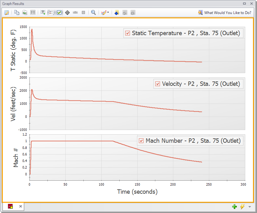
Figure 31: The Graph Results window offers full-featured plot generation. The static temperature, velocity, and Mach number of Pipe P2 outlet are shown.
Further review of the graph results in Figure 31 shows that sonic choking occurs after several seconds
Note: AFT xStream assumes all pipes are adiabatic (perfectly insulated). Over a 240 second run time this assumption may not be accurate. Consider this when evaluating simulation results over longer times.
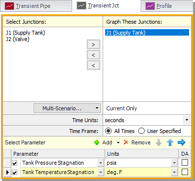
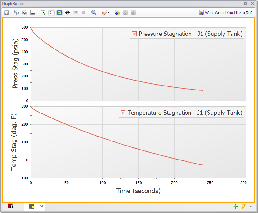
Figure 33: The Transient Junction graph shows how variables within a junction change over time. The temperature and pressure of Tank J1 over time are plotted.
This junction graph could be used to determine when certain conditions within the tank were met. For instance, suppose there was a need to know when the tank pressure dropped below
Lastly, we will animate the profile of the Blowdown Tank system to show the wave caused by opening the valve. In the Quick Access Panel, open the Profile tab. Under Plot Single Path, select Pipe 1 and Pipe 2. After ensuring your length is
ØClick the Generate button. This will show an animated profile of the pipe system over the specified time frame (see Figure 35).

Figure 35: The Profile Graph show the Maximum and Minimum values of all parameters shown in the Graph over the specified time Frame. It can also be set to animate the values so that the behavior within the system as a whole can be observed. The blue line correlates to minimum values, the bright red line shows maximum value, and the dark red line shows the value at the current timestep.
Take note of the pressure wave that is created at the valve just after animation is started. This wave travels to the Assigned Pressure junction before reflecting back towards the valve. The amount of time it takes this wave to travel to the reflection point and back is called the communication time. It should be noted when creating your transient that any event that occurs over a shorter length of time than the communication time of the system is considered to happen instantaneously.
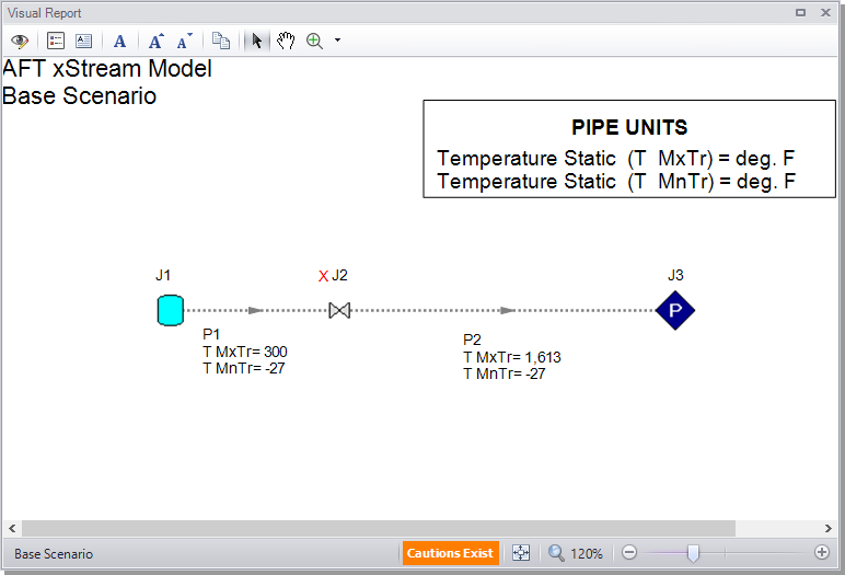
C. View the Visual Report
The Visual Report allows you to show text output alongside the model schematic. This is useful to quickly show pertinent information in relation to location in the model. The Visual Report can also animate the transient pipe results in a color animation overlaid on the model.
-
ØChange to the Visual Report window by choosing it from the Window menu, clicking the Visual Report tab or by pressing Ctrl+I. The Visual Report window allows you to integrate your text results with the graphic layout of your pipe network. The Visual Report Control window should open automatically when accessing the Visual Report window for the first time. The Visual Report Control window can also be opened from the Visual Report Toolbar or the Tools menu. Note that the parameters present in Visual Report Control are determined by the parameters selected in Output Control.
-
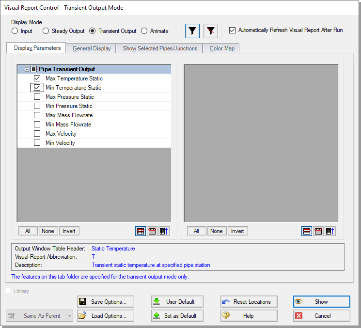
ØSelect "Max Temperature Static" and "Min Temperature Static" in the Pipe Transient Output area of the Visual Report Window as shown in Figure 36. Click the Show button. This will generate the Visual Report window graphic seen in Figure 37.
It is common for the text in the Visual Report window to overlap when first generated. You can change this by selecting smaller fonts or by dragging the text to a new area to increase clarity. You can also use the Visual Report Control window to display units in a legend to increase the clarity of the display. These adjustments have already been done in Figure 37. This window can be printed or copied to the clipboard for import into other Windows graphics programs, saved to a file, or printed to an Adobe PDF file.
D. Examine the Effect of Heat Transfer
By default AFT xStream models all pipes as adiabatic at the internal surface, meaning no heat is transferred from the fluid to the pipe walls or surroundings. Modeling the pipes as adiabatic is reasonable when the pipes are well insulated and the temperature difference between the fluid and the atmosphere is relatively low. However, for cases such as the tank blowdown modeled in this example heat transfer from the fluid to the pipe walls and environment has a large impact on results.
To see the impact of convective heat transfer on the results create a child scenario named “Convective Heat Transfer.”
In the “Convective Heat Transfer” scenario update pipes P1 and P2. Open the Pipe Properties window for each pipe and enter the following on the Heat Transfer tab (Fig):
-
Heat Transfer Model = Convective Heat Transfer
-
External Convection Coefficient Correlation = Free-Horizontal (Churchill-Chu)
-
Ambient Temperature =
After updating each of the pipes open the Analysis Setup window and go to the Pipe Sectioning and Output panel. Change the Estimated Maximum Pipe Fluid Temperature During Transient to
ØRun the model and go to the Output window.
In the Transient Max/Min tab shown in Figure 38 it can be seen that the maximum temperature in pipe P2 is only
Go to the Graph results window and recreate the pipe P2 outlet graph from Figure 31 as is shown below in Figure 39.
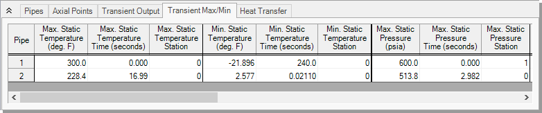
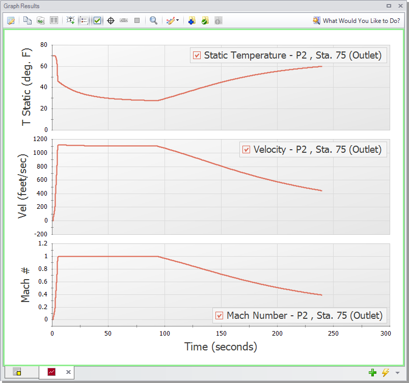
Figure 39: Temperature, velocity, and Mach number for the discharge of Pipe P2 with convective heat transfer
E. Examine the Effect of Sectioning
In AFT xStream, sectioning plays an important role in model accuracy. Due to how the MOC operates, accuracy increases with the number of sections you have in the model. To illustrate this, the model was re-run with a Minimum Number of Sections Per Pipe of 6. Comparing Figure 33 to Figure 42, values such as the tank temperature and pressure for Tank J1 remain similar with the increase in the number of sections. However, values such as the maximum temperature reached in Pipe 2 (Figure 25 and Figure 40), changed substantially. This value increased from
Due to the long run time, it was not sensible to ask you to run the 6 section scenario as a part of this example. If you are interested, you may want to run this scenario overnight.
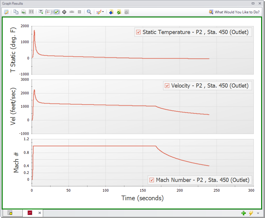
Figure 41: Temperature, velocity, and Mach number for the discharge of Pipe P2 with 6 sections minimum per pipe

Figure 43: Profile Graph for Tank Blowdown system with 6 Sections Minimum Per Pipe where the blue line represents the minimum value, the bright red line represents the maximum value and the dark red line represents the value at the current time step
Conclusion
You have now used AFT xStream's five Primary Windows to build and analyze a simple gas transient model.