Method of Characteristics
The Method of Characteristics is a general approach for solving a partial differential equation by reducing it to a system of ordinary differential equations.
We see here how it is applied to the transient flow equations. The three partial differential equations have three unknowns P,V, and ρ, and two independent variables x and t. Application of the Method of Characteristics will generate six ordinary differential equations.
Characteristic Equations
First linearly combine the equations with the introduction of constant factors represented by λ:

Note that for the above equation, the area was assumed to be constant, so all partial derivatives with respect to A were dropped to simplify the equation.
Rearranging terms from the linear combination above

We define relationships for λ1, λ2, and λ3:


By asserting that λ3 = 1, it is found that

and

Substituting into the above equation:

We have three solutions for λ, each valid along a certain characteristic line, as will be described further below. The solutions are as follows

This represents the six characteristic equations that we are searching for, paired as the right running (R), left running (L), and particle path (P) sets of equations:

where

The relationship between the time step, length step, sonic velocity and velocity from the characteristic equations shown here is crucial for effectively sectioning the pipes, which is discussed further in Pipe Sectioning - Introduction to Method of Characteristics.
Note: This set of ordinary differential equations represent an exact solution to the governing equations, given the minor assumptions that flow is one dimensional, gravity does not change in time and space, and the pipe is rigid and constant area.
Numerical Method
We can simplify the equations further into a form that is convenient for simulation.
For each of the equations multiply by dt as is shown below for the right running characteristic

This equation can be integrated along the right running characteristic.
It is useful at this stage to consider a graphical representation of the characteristic grid.
On the characteristic grid point 4 will be affected by the right running characteristic from point R, the left running characteristic from point L, and the particle path characteristic from point P.
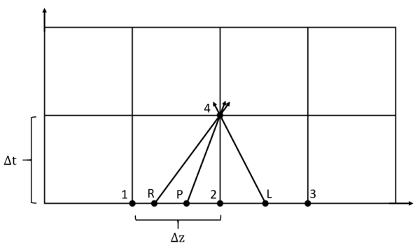
Figure 1: Characteristic grid. The point 4 sees effects from points R, L, and P after some time dt, which has equal magnitude of dx/a
Setting up the integral along the right running characteristic line:

This integrand represents the exact solution. However, in order to evaluate the integral, several major assumptions will be made:
-
The values are only known at the grid points (points 1, 2, and 3 in Figure 1). Therefore, interpolation is required to find the values at points R, L, and P. In literature this is often cited as the largest source of error. Linear interpolation is used to determine the position, z, and the properties at each of the starting points R, L, and P. Though compressible flow properties do not vary linearly along a pipe, it has been found that more sophisticated interpolation is less stable and requires a much larger calculation time, which is why linear interpolation is used for xStream.
-
The variables in each integrand cannot all be related, so an analytical solution cannot be found for each of the integrals. Instead, the integrands are assumed to be constant, using the values from the starting point. In some cases this may be a good approximation, as the properties are relatively constant. However, in other cases, such as at high Mach numbers, the properties would change rapidly in reality. Adding additional sections helps reduce error caused by this assumption.
-
Related to the constant integrand and interpolation assumptions, the characteristic lines are assumed to be straight. In reality the slope would constantly change as both the velocity and sonic velocity are changing over time. Assuming the characteristic lines are straight allows the starting points R, L, and P to be interpolated as discussed above.
Using the 3 assumptions above, the integral is trivial, and the below solution can be found for the right running characteristic:

where

We can repeat the above process for the left running characteristic and particle path characteristic to arrive at:


where


We have finally arrived a system of three equations with only three unknowns - pressure, density and velocity at point 4. These equations can be further arranged into a convenient form known as the compatibility equations.