Pipe Sectioning - Introduction to Method of Characteristics
To run any transient simulation in AFT xStream, the pipes in the model must first be sectioned. This is required to use the Method of Characteristics (MOC) solution approach. A brief overview of the impact the Method of Characteristics has on the model is covered below. A detailed discussion on the mathematics behind the method is covered on the Method of Characteristics help topic.
What is Sectioning?
The Method of Characteristics requires the entire system to be solved every time step. To accomplish this, every section must use a common time step. If the time steps were allowed to vary throughout the model, some portions of the system would be solved "ahead" of others, resulting in a time-distorted solution.
Furthermore, the Method of Characteristics requires that any information propagated from a given calculation point arrives at the neighboring calculation points after one time step. The method cannot allow information to be "lost" between time steps or calculation stations - the distance between calculation points is locked to the duration of a time step.
The time Δt it takes to travel from one point to another is determined by the linear distance Δx between those points and the wave velocity (a + V):

For systems with liquid flow the velocity is relatively small and can be neglected, which results in a constant characteristic line slope:

However, for gas flow the velocity cannot be neglected, which means that the characteristic line slope will change throughout the transient. This complicates the choice of a characteristic grid size, since the AFT xStream MOC solution requires a fixed grid. For a fixed time step, the distance the wave travels will vary based on the wave velocity at that time step. Interpolation must be performed between the known grid points to determine the unknown pressure, velocity, and temperature at time step t in order to calculate the pressure, velocity, and density at time step t + Δt at the grid intersection.
For example, consider Figure 1 below where the parameters at point 4 are being determined. At time step t, points 1, 2, and 3 are known from the previous MOC calculation. However, based on the wave velocity at time step t the characteristic lines will be unlikely to fall on the known grid points, so interpolation must be performed. Ideally the points R, P, and L will fall between points 1 and 3 on the grid for a stable solution.
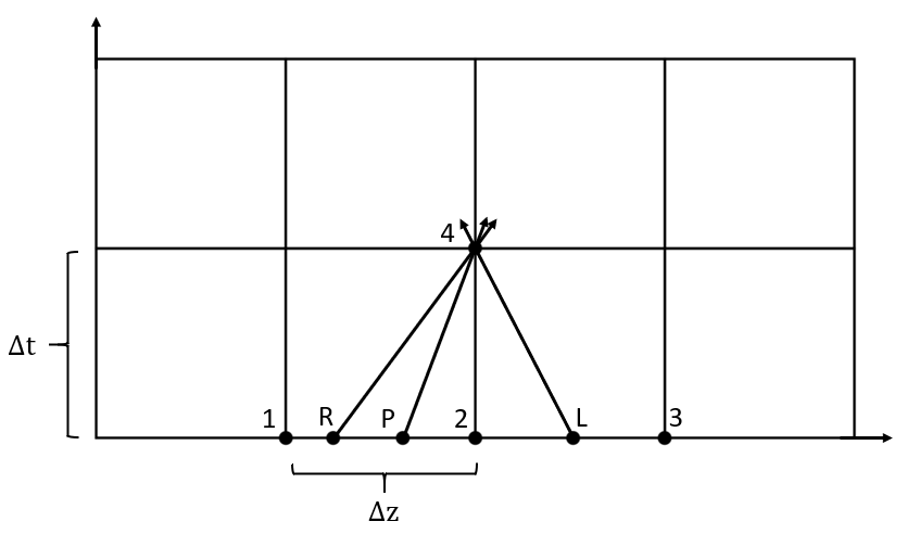
Figure 1: Characteristic grid in AFT xStream, where point 4 sees effects from points R, P, and L after some time dt, which has equal magnitude of dx/a. Points R, P, and L must be interpolated from know points 1, 2, and 3.
To ensure that grid points 1 and 3 are not exceeded the minimum time step can be approximated using the maximum value of a + V. Recall that the maximum velocity for gas flow in a pipe is limited to the sonic velocity, and that the maximum sonic velocity will occur at the maximum temperature (T,max). Therefore, the minimum time step can be calculated as follows:

Note: The maximum temperature during the transient will likely be unknown when the model is first run. It is best practice to choose a conservatively large temperature when first running the model. The maximum temperature can be decreased for subsequent runs to increase the accuracy of the results as necessary.
Note that the multiplier of 2 for the maximum sonic velocity, known as the courant factor, was derived assuming that the velocity reaches the sonic velocity (Mach number reaches 1). If the Mach number does not reach 1 during the transient simulation, then using two times the maximum sonic velocity will be an overestimate for the maximum velocity. This large maximum velocity allows for a stable solution, but also reduces the accuracy of the solution since points R and L are farther away from the grid points 1 and 3.
For simulations where the Mach number in the pipes remains significantly below one for the whole duration the accuracy can be increased by decreasing the courant factor, which should be equivalent to one plus the maximum pipe Mach number. Calculating the courant factor using a Mach number less than the maximum pipe Mach number will result in an unstable solution and may prevent the MOC from converging.
Note: In xStream the courant factor is adjusted based on the Estimated Maximum Pipe Mach Number During Transient defined in the Sectioning panel of Analysis Setup. By default the Estimated Maximum Pipe Mach Number is fixed at 1, and can only be changed if advanced options are enabled.
Sectioning Effect on Accuracy
One of the largest sources of error in xStream results from the interpolations performed to determine the properties at points R, P, and L. To increase the accuracy of calculations the width between the grid points, Δx, can be reduced by increasing the minimum number of sections. For a detailed discussion on determining result accuracy, see the Transient Results Accuracy topic.
Sectioning Effect on Run Time
As is discussed above, the accuracy of the results in xStream will be closely tied to the number of calculation sections. However, the more calculation stations there are, the longer the required run time will be. xStream simulation times may require hours or days to run, depending on the size of the model and the computational speed of the computer. For information on reducing run times see the Minimizing Run Time topic.
Related Topics


