Natural Gas Burner - ANS (English Units)
Natural Gas Burner - ANS (Metric Units)
Summary
This example will size the pipes for a natural gas supply system to five burners. It is desired to analyze two separate design cases using monetary cost automated sizing.
Note: This example can only be run if you have a license for the ANS module.
Topics Covered
-
Sizing using monetary cost
-
Using dependent design cases to satisfy two different operating modes for a system
-
Understanding the effect of monetary vs. non-monetary sizing objectives
Required Knowledge
This example assumes the user has already worked through the Beginner: Air Heating System example, or has a level of knowledge consistent with that topic. You can also watch the AFT Arrow
In addition, it is assumed that the user has worked through the Beginner: Three Tank Steam System - ANS example, and is familiar with the basics of ANS analysis.
Model Files
This example uses the following files, which are installed in the Examples folder as part of the AFT Arrow installation:
-
Steel - ANSI Pipe Costs.cst - cost library for Steel - ANSI pipes
Step 1. Start AFT Arrow
From the Start Menu choose the AFT Arrow 9 folder and select AFT Arrow 9.
To ensure that your results are the same as those presented in this documentation, this example should be run using all default AFT Arrow settings, unless you are specifically instructed to do otherwise.
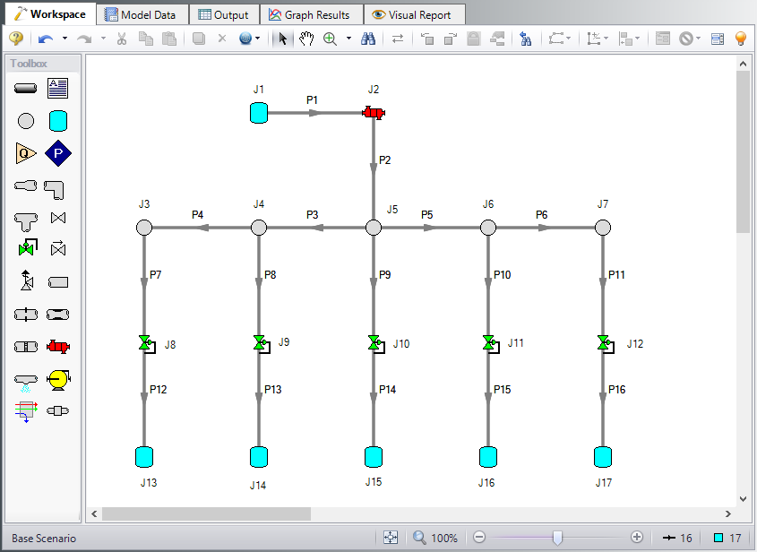
Open the US - Natural Gas Burner - ANS Initial.aro example file listed above, which is located in the Examples folder in the AFT Arrow application folder. Save the file to a different folder. The Workspace should look like Figure 1 below.
Step 2. Define the Modules Group
Navigate to the Modules panel in Analysis Setup. Check the box next to Activate ANS. The Network option should automatically be selected, making ANS enabled for use.
Step 3. Define the Automatic Sizing Group
For this system we will be sizing the natural gas system for two different operating cases, one with all burners running and one with the third burner closed. When modeling multiple design cases, the different cases need to be broken up into a primary design case, of which there is one, and dependent design cases, of which there can be any number.
The primary design case can be any of the design cases that are being addressed in your model. Typically, it will represent the primary operating condition of the pipe system. If it is not clear which case should be the primary case, just pick any of the cases and call that the primary one. Design cases other than the primary case are referred to as dependent design cases. This naming convention is used since the dependent design cases are built and defined by duplicating the primary design case, as will be discussed later. The case with all burners on will be used as the primary design case.
To start we will set up the sizing settings for the primary design case, after which we will set up the dependent design case.
A. Sizing Objective
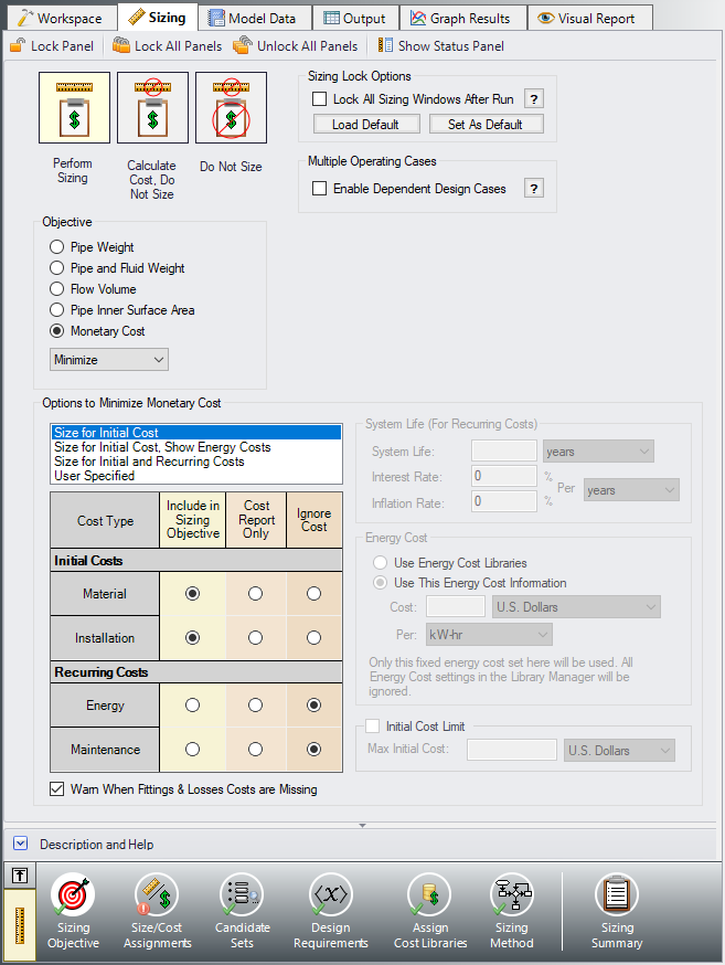
The Sizing Objective panel should be selected by default. For this analysis, we are interested in sizing considering the monetary cost for the initial costs only.
-
Set the Sizing Option to Perform Sizing.
-
For the Objective, choose Monetary Cost, and select the Minimize option from the drop-down list.
-
Under Options to Minimize Monetary Cost, choose Size for Initial Cost. This will update the cost table to include both initial costs in the sizing calculation while ignoring the recurring costs.
The Sizing Objective window should now appear as shown in Figure 2.
B. Size/Cost Assignments
On the toolbar at the bottom of the window select the Size/Cost Assignments button.
For the supply lines P1 and P2, the pipe size is fixed to 6 inches and will not be sized. However, we will still need to purchase these pipes, so we will consider their cost. The rest of the pipes in the system will need to be sized for the design.
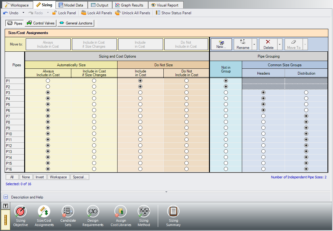
The 4 header pipes (P3, P4, P5, P6) represent a single header in the physical system, so it will be necessary to add them to a Common Size Group. A second Common Size Group should be created to contain all of the discharge piping (P7 - P16), as each of the branches to the burners should be identical. To set up the Size/Cost Assignments as described, do the following:
-
Move pipes P1 & P2 to Do Not Size – Include in Cost in the table. This will calculate their cost while keeping their size fixed.
-
Select pipes P3 - P16 in the table by holding SHIFT to select multiple rows, then click the Always Include in Cost button to move them to the appropriate column to be sized.
-
Now that the pipes have been set to be sized, the Common Size Groups need to be created. Select New above the Pipe Grouping table to create two new groups and give them the names Headers and Distribution.
-
Add pipes P3 - P6 to the Headers group using the radio buttons. Alternatively, they can be added by selecting the pipes in the Workspace then right-clicking and choosing the appropriate option to add them to the group.
-
Add pipes P7 - P16 to the Distribution group either by using the radio buttons in the table, or from the Workspace.
The Size/Cost Assignments table should now appear as shown in Figure 3.
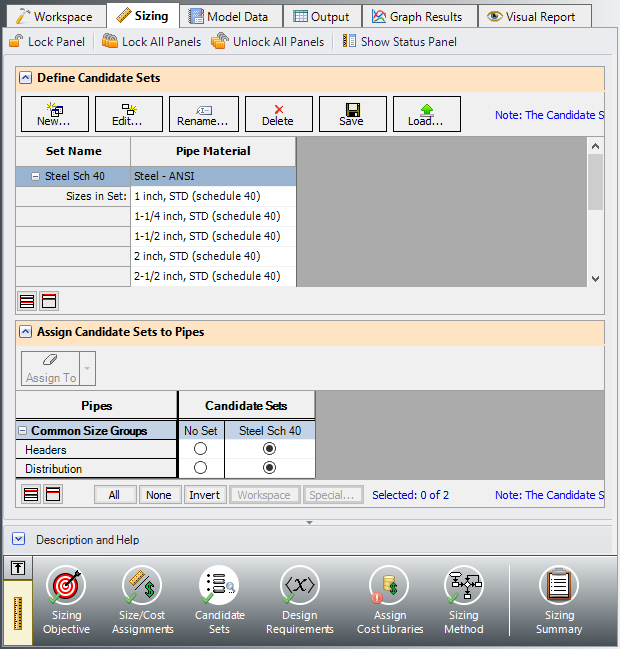
C. Candidate Sets
Click on the Candidate Sets button to open the Candidate Sets window. In this case we will be considering schedule 40 steel pipe within the range of 1" - 12".
-
Select New, and name the Candidate set Steel Sch 40.
-
Choose Steel - ANSI from the material list.
-
Expand the STD type, then double click each of the sizes from 1 inch to 12 inch to add them to the Candidate Set.
-
Click OK to accept the defined set.
In the bottom section of the window make sure that the Common Size Groups are assigned to use the new Steel Sch 40 Candidate Set. The window should appear as shown in Figure 4.
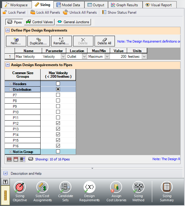
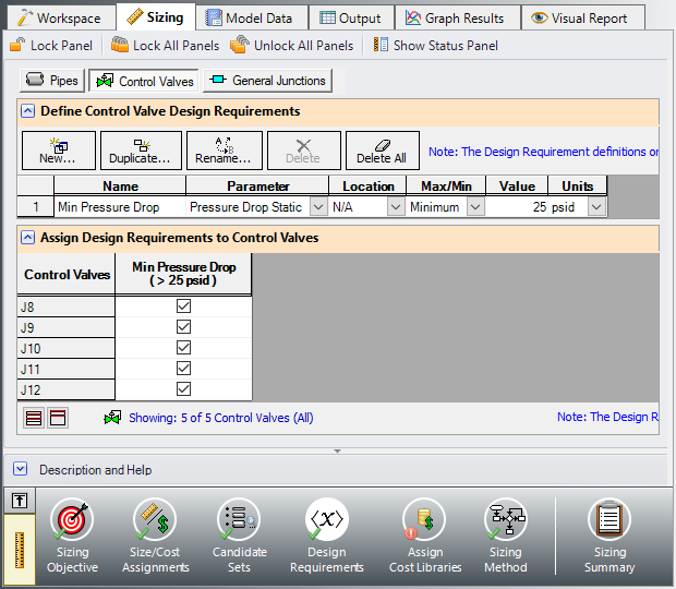
D. Design Requirements
Select the Design Requirements button.
In the primary design case the following requirements need to be met:
-
The flow to the burners must remain below the maximum velocity requirement of
-
All control valves must have a minimum pressure drop of
Make sure that the Pipes button is selected, then create a new Design Requirement named Max Velocity specifying the Velocity Outlet Maximum of the pipe is
Next select the Control Valves button at the top of the window and create a new control valve Design Requirement. Name the Design Requirement Min Pressure Drop, and specify the Pressure Drop Static as a Minimum of
E. Assign Cost Libraries
Select the Assign Cost Libraries button. For this model the pipe cost library has already been created, but we will need to connect and apply it.
ØOpen the Library Manager by clicking the Library Manager button to see which libraries are connected.
This example uses a pre-built cost library for the pipes containing the Steel material costs. To connect the library do the following:
-
Click the button Add Existing Cost Library.
-
Browse to the AFT Arrow 9 Examples folder (located by default in C:\AFT Products\AFT Arrow 9\Examples\), and select the file titled Steel - ANSI Pipe Costs.cst.
The new library should now be visible in the Available Libraries list, be automatically connected to the model, as shown in Figure 7. The cost library for the pipes should appear with the name Steel - ANSI Pipe Costs and be indented under the Steel - ANSI library within the standard pipe material libraries list.
Once you have confirmed that the library is connected, click Close to exit the Library Manager.
Back in the Assign Cost Libraries panel for the Pipes the Steel - ANSI Pipe Costs library should be the only available cost library, and should be selected to show that it is being applied to the candidate sets and to each of the supply lines as shown in Figure 8.
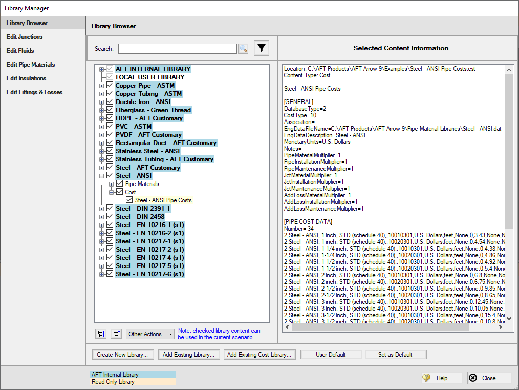
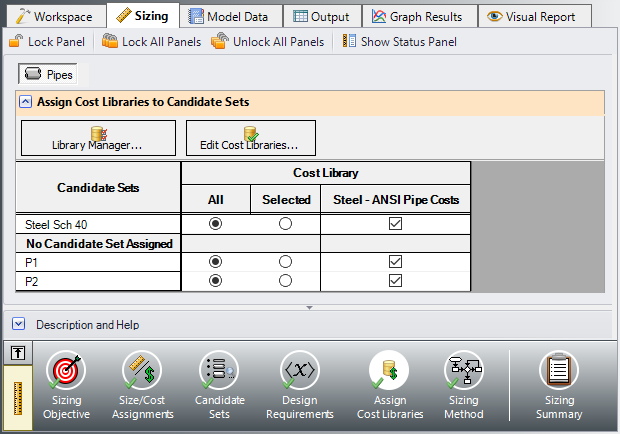
Figure 8: Assign Cost Libraries panel with the Steel - ANSI Pipe Costs library connected and applied to the pipes in the model
F. Sizing Method
Select the Sizing Method button to go to the Sizing Method panel.
Ensure that Discrete Sizing is chosen with the Modified Method of Feasible Directions (MMFD) for the Search Method.
G. Dependent Design Cases
We have now set up the system to be sized for the primary design case, but we will also need to account for the case where the third burner is shut off. There are a few changes that will need to be made for this additional case:
-
The flow rate at the control valves increases to
-
Control Valve J110 is closed and the minimum design requirement is removed because it is shut off.
To make the dependent design case where the third burner is shut off complete the following:
-
Go to the Sizing Objective panel and select the Enable Dependent Design Cases option. A new button will now be available for the Dependent Design Cases panel in the Sizing Navigation panel.
-
Navigate to the Dependent Design Case panel. You should now see instructions displayed to create Dependent Design Cases, along with a summary table of dependent design settings. We will now need to use the Duplicate Special feature to create the dependent design case.
-
Go to the Workspace and choose Select All from the Edit menu.
-
Open Duplicate Special (from the Edit menu), enter an increment of 100 and select Make Dependent Design Case (Figure 9). Click OK.
-
Move the duplicated pipes and junctions to distinguish them from the original ones in the Primary Design Case.
-
Close Control Valve J110 in the DDC by selecting the junction in the Workspace and clicking the Special Conditions button
 on the Toolbar and selecting Closed.
 -
Use Global Junction Edit (from the Edit menu) to change all of the control valve setpoints in the DDC from
-
In the Sizing window navigate to the Design Requirements panel. On the Control Valves page remove the pressure drop requirement from J110, since this valve is closed for the DDC.
Return to the Dependent Design Cases panel.
When Duplicate Special was performed with Dependent Design Case selected, each of the duplicated pipes was created with a special type of grouping. For example, pipe 101 is grouped with pipe 1 as a DDC pipe (see Figure 11). This type of assignment allows the dependent design pipes to be sized, but to not be counted in the cost so that the cost will not be duplicated.
It should also be noted that the dependent design grouping causes each of the dependent pipes to inherit their Common Size Groups, Candidate Sets, and Cost Library settings from the pipes in the primary case. The dependent design case pipes are therefore hidden on all sizing panels except for the Design Requirements and Dependent Design Cases panels.
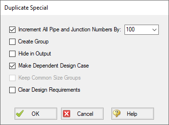
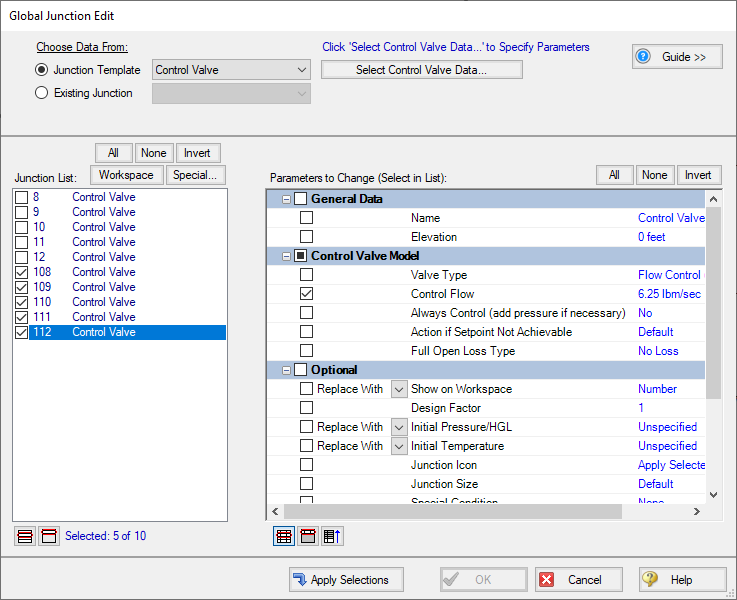
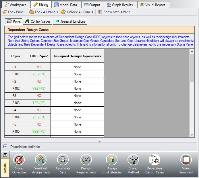
Figure 11: Pipes in Dependent Design Cases have a special grouping relationship with pipes in the primary case
Step 4. Run the Model
Click Run Model on the toolbar or from the Analysis menu. This will open the Solution Progress window. This window allows you to watch as the AFT Arrow solver converges on the answer. Once the solver has converged, view the results by clicking the Output button at the bottom of the Solution Progress window.
Step 5. Examine the Output
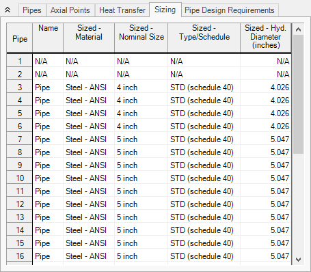
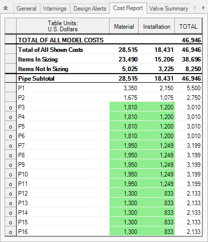
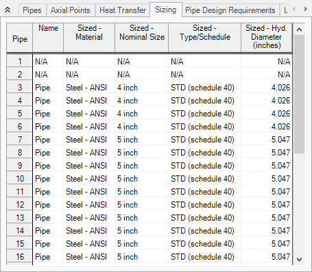
After the run finishes, examine the final pipe sizes calculated by the ANS module. The results for pipe size and overall cost are shown in Figure 12 and Figure 13. One can see that the resultant size is 4-inch pipe for the header, with larger 5-inch piping for the distribution lines.
The total cost for the pipes is $46,946. This includes the $8,250 cost for the supply line pipes which were not sized, as well as the $38,696 cost for the pipes in the model which were sized, including the header and distribution piping. The pipes that were sized will be distinguished in the Cost Report by having a green background color.
Step 6. Compare Results With Non-Monetary Sizing
This sizing could be performed by using weight as the objective instead of monetary cost to simplify the setup. Using a non-monetary objective can produce less accurate sizing results in cases where the energy costs or costs of equipment such as compressors need to be accounted for. However, only the pipe sizes are being considered for the sizing calculations in this example. Set up the model to perform a non-monetary sizing by doing the following:
-
In the Scenario Manager create a child of the Base Scenario by right-clicking the scenario name and choosing Create Child.
-
Give the new child scenario the name Pipe Weight Sizing.
-
Go to the Sizing Objective panel and change the Objective from Monetary Cost to Pipe Weight.
The model should now be configured to run the model. Click Run Model, then go to the Output window once the run is finished. The final pipe sizes should now appear as shown in Figure 14.
It can be seen that changing the objective to pipe weight produces identical sizing results as the run using a monetary cost objective. For more complex systems this will not always be the case.