Process Steam System - ANS (Metric Units)

Summary

This example sizes a process steam system by minimizing the pipe weight. Common Size Groups allow for the system to be simplified while still effectively sizing the system.

Note: This example can only be run if you have a license for the ANS module.

Topics Covered

• Defining Common Size Groups

• Viewing Common Size Groups using color in the Workspace

• Choosing a Search Method

Required Knowledge

This example assumes the user has already worked through the Beginner: Air Heating System example, or has a level of knowledge consistent with that topic.  You can also watch the AFT Arrow Quick Start Video (English Units) on the AFT website, as it covers the majority of the topics discussed in the Beginner: Air Heating System example.

In addition, it is assumed that the user has worked through the Beginner: Three Tank Steam System - ANS example, and is familiar with the basics of ANS analysis.

Model Files

This example uses the following files, which are installed in the Examples folder as part of the AFT Arrow installation:

• US - Process Steam System.aro

• US - Process Steam System - ANS.aro

Step 1. Start AFT Arrow

From the Start Menu choose the AFT Arrow 9 folder and select AFT Arrow 9.

To ensure that your results are the same as those presented in this documentation, this example should be run using all default AFT Arrow settings, unless you are specifically instructed to do otherwise.

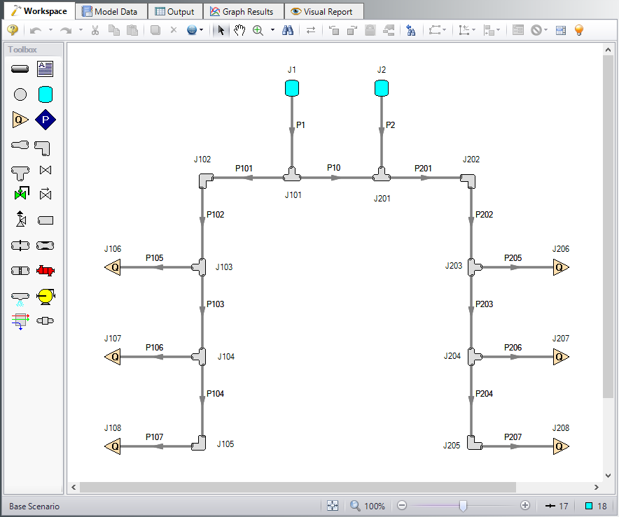
Open the US - Process Steam System.aro example file and save it to a new location. Open the newly saved model file, right-click on the Base Scenario and select Delete All Children. The Workspace should look like Figure 1 below.

Step 2. Define the Pipes and Junctions Group

Before running this model with ANS, change all Tee/Wye junctions to use the Simple (no loss) Loss Model rather than the Detailed Loss Model. This is significantly reduce the complexity of the model and allow the solver to converge much faster. Use Global Junction Edit to make this change.

Step 3. Define the Modules Group

Navigate to the Modules panel in Analysis Setup. Check the box next to Activate ANS. The Network option should automatically be selected, making ANS enabled for use.

Step 4. Define the Automatic Sizing Group

The model is already defined for a regular AFT Arrow run, but we need to complete the sizing settings before running the analysis. Go to the Sizing window by clicking the Sizing tab.

A. Sizing Objective

Go to the Sizing window by selecting the Sizing tab. The Sizing Objective window should be selected by default from the Sizing Navigation panel along the bottom. For this analysis, we are interested in sizing the system considering the monetary cost for the initial costs only.

1. Select Perform Sizing for this calculation.

2. For the Objective, choose Pipe Weight, and select the Minimize option from the drop-down list.

The Sizing Objective window is now complete.

B. Sizing Assignments

On the Sizing Navigation panel select the Sizing Assignments button.

For this system, we will be sizing all of the pipes since it is a new system.

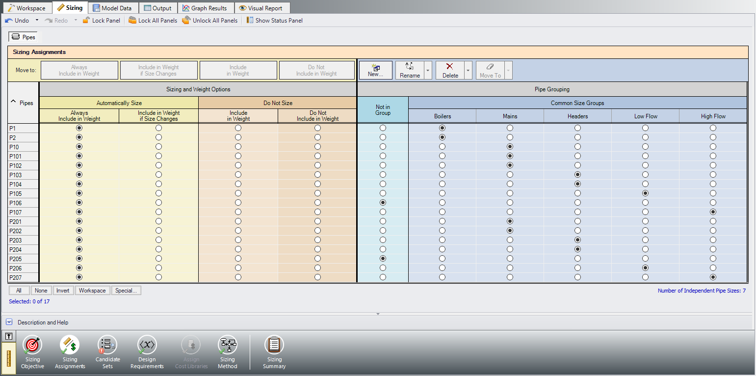
ØMove all of the pipes to Always include in Weight.

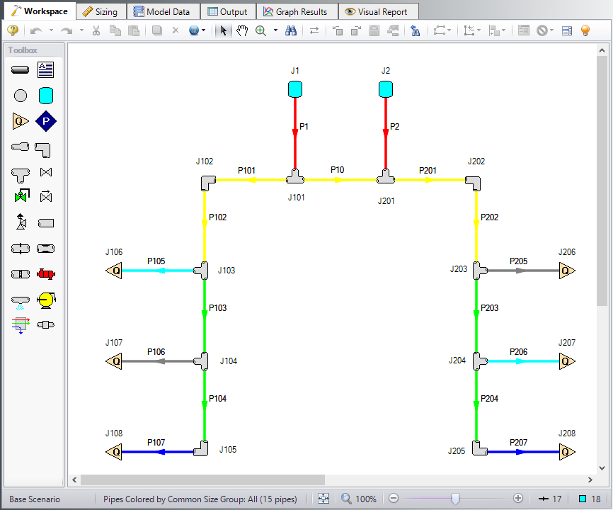
To more efficiently size the system, it would be beneficial to create common size groups. In this system there are several sections of piping which would likely be grouped together. Create Common Size Groups as described below and indicated by the colors in Figure 2.

1. The boilers in the model are identical, so it would be logical to use equivalent pipe sizes for pipes P1 and P2 connected to the boilers. Create a Boilers Common Size Group and add pipes P1 and P2 to the group.

2. Using a common pipe size for the headers would be desirable in this system to reduce installation costs and reduce losses. However, grouping the headers downstream of users 1 and 4 separately could allow us to use a smaller size for those pipes and save costs. Create two groups, Mains and Headers as shown in yellow and green respectively in Figure 2.

3. In this system the users have varying flow demands, so it is not desirable to use a common pipe size for all of the users. However, several of the users do have identical flows, so the pipes connected to those users should be grouped. Create a Low Flow Users group for pipes P105 and P206 and a High Flow Users group for pipes P107 and P207.

The completed pipe Sizing Assignments can be seen in Figure 3.

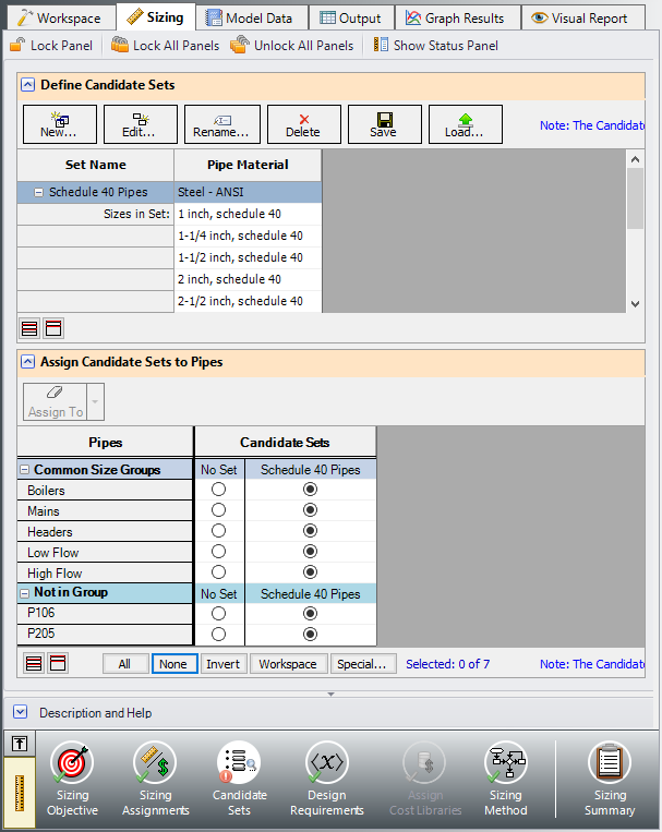
C. Candidate Sets

Click on the Candidate Sets button to open the Candidate Sets panel.

For this system it is desired to use STD Steel - ANSI. To create a Candidate Set, do the following:

1. Under Define Candidate Sets, click New.

2. Give the set the name Schedule 40 Pipes and click OK.

3. From the drop down list choose Steel - ANSI.

4. In the Available Material Sizes and Types on the left, expand the schedule 40 pipe sizes list.

5. Double-click each of the sizes from 1 to 12 inches to add them to the list on the right.

6. In the Select Pipe Sizes window, click OK.

We now need to define which pipes will use this Candidate Set during the sizing calculation. Check the boxes next to each of the pipes and Common Size Groups to assign the Candidate Set to each of the pipes, as shown in Figure 4.

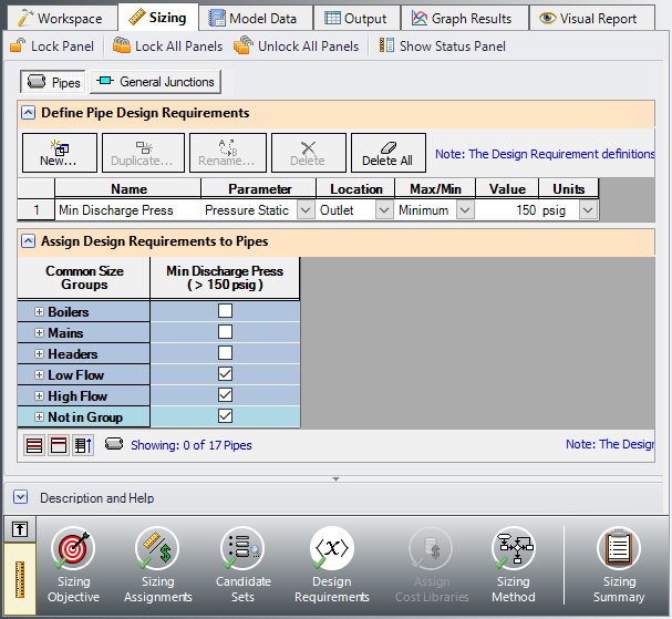
D. Design Requirements

Select the Design Requirements button from the Navigation Panel.

For this system there is a requirement to maintain a minimum discharge pressure of 150 psig to each of the customers. Design Requirements can not be applied on the assigned flow junctions directly, so we will define this requirement at the outlet of each of the pipes connected to the Assigned Flow junctions.

1. Click the New button under Define Pipe Design Requirements.

2. Enter the name Min Discharge Press.

3. Select Pressure Static as the Parameter.

4. Set the Location as Outlet.

5. Choose Minimum for Max/Min, and enter 150 psig.

Now we need to apply the defined Design Requirement to the discharge pipes.

ØCheck the box next to each of the discharge pipes in the Assign Design Requirements to Pipes section. This can be done quickly by checking the boxes next to the two Common Size Groups and the Not in Group header to select all of the  pipes under those classifications. The Design Requirements panel should now appear as shown in Figure 5.

E. Assign Cost Library

When the Sizing Objective has been defined as monetary cost, it is necessary to create and assign cost libraries for the automated sizing, which can be done in the Assign Cost Library panel. Since we have defined the objective as Pipe Weight, we will not need to assign any cost libraries, and this button is disabled.

F. Sizing Method

Select the Sizing Method button to go to the Sizing Method panel.

ØChoose Discrete Sizing, since it is desired to select discrete sizes for each of the pipes in the model.

For the search method, the ANS module suggests using the Modified Method of Feasible Directions, so select that option from the Search Methods list. Note that the suggested method will be displayed if the Suggest Best Method button is selected under the Search methods list.

Step 5. Run the Model

Click Run Model on the toolbar or from the Analysis menu. This will open the Solution Progress window. This window allows you to watch as the AFT Arrow solver converges on the answer. Once the solver has converged, view the results by clicking the Output button at the bottom of the Solution Progress window.

Step 6. Examine the Output

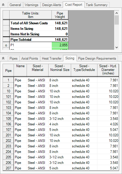
After the run finishes, examine the final pipe sizes calculated by the ANS module. The results for pipe size and overall cost are shown in Figure 6. The resultant pipe sizes range from 3-1/2 to 10 inches throughout the system.

With the Modified Method of Feasible Directions the total pipe weight in the system is minimized to 148,621 lbm.

For this system it is possible to further minimize the weight in the system by using the Genetic Algorithm (GA) method. With Genetic Algorithm a further reduction of about 5,000 lbm can be obtained, though the run time is much longer. Note that it is possible to pause the solver and accept the current sizing solution before the Genetic Algorithm has fully completed by clicking Pause, then selecting Accept Sizing from the Other Actions menu and clicking Continue to finish the current iteration. This will provide a valid system design, though it may not be the best solution that could possibly be found.

For more complex models this additional run time may be much longer, but could potentially provide a larger amount of savings. The main product Help file provides more information on setting up the model to use the Genetic Algorithm Search Method.