Beginner: Three Reservoir Example (English Units)
Beginner: Three Reservoir Problem (Metric Units)
Summary
This example provides an overview of AFT Fathom's layout and structure. The basic features will be used to build a three-pipe, four-junction model to solve the classic three-reservoir problem.
Topics Covered
-
Drawing the system with pipes and junctions
-
Entering pipe and junction properties
-
Completing Analysis Setup
Required Knowledge
No previous experience with AFT Fathom is required to complete this example. It begins with the most basic elements of laying out the pipes and junctions and solving the system hydraulics with the Newton-Raphson methodology.
Model File
This example uses the following file, which is installed in the Examples folder as part of the AFT Fathom installation:
Step 1. Start AFT Fathom
ØTo start AFT Fathom, click Start on the Windows taskbar, choose AFT Fathom 12, and launch the program. (This refers to the standard menu items created by setup. You may have chosen to specify a different menu item during installation).
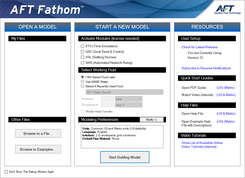
As AFT Fathom starts, the start-up screen, as shown in Figure 1, appears with several options before to start building a model. Some of the actions available are:
-
Open a recent model, browse to a model file, or browse to an Example
-
Activate an Add-on Module
-
Select ASME Water or a recently used fluid to be the Working Fluid
-
Review or modify Modeling Preferences
-
Select a Unit System
-
Filter units to include Common Only or Common Plus Selected Industries
-
Choose a Grid Style
-
Select a default Pipe Material
-
-
Access other Resources, such as Quick Start Guides, Help Files, and Video Tutorials
Note: If you are working through the Metric Units version of the Examples, be sure to specify either Metric Only or Both with Metric Defaults as the unit set by modifying the Modeling Preferences.
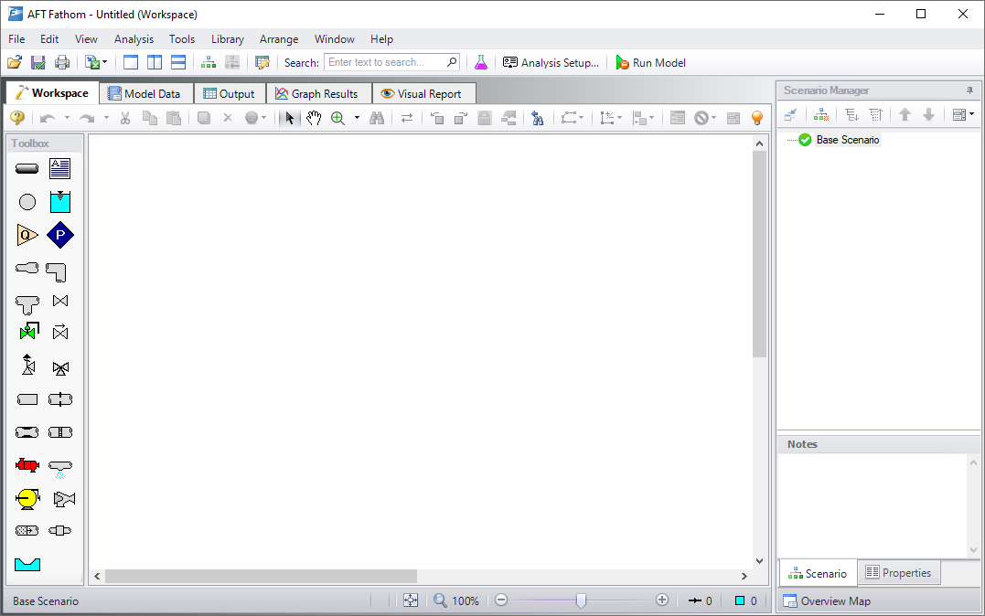
After clicking the Start Building Model button on the start-up window, the Workspace window is initially always the active (large) window, as seen in Figure 2. The five tabs in the AFT Fathom window represent the five primary windows. Each Primary Window contains its own toolbar that is displayed directly beneath the Primary Window tabs.
AFT Fathom supports dual monitor usage. You can click and drag any of the five primary window tabs off of the main AFT Fathom window. Once you drag one of the primary windows off of the AFT Fathom window, you can move it anywhere you like on your screen, including onto a second monitor in a dual monitor configuration. To add the primary window back to the main Fathom primary tab window bar, simply click the red X button in the upper right of the primary window.
To ensure that your results are the same as those presented in this documentation, this example should be ran using all default AFT Fathom settings, unless you are specifically instructed to do otherwise.
The Workspace window
The Workspace window is the primary vehicle for building your model. This window has three main areas: the Toolbox, the Quick Access Panel, and the Workspace itself. The Toolbox is the bundle of tools on the far left.
The Quick Access Panel is on the right. It is possible to minimize the Quick Access Panel by clicking on the thumbtack pin in the upper right of the Quick Access Panel in order to allow for greater Workspace area.
The Workspace takes up the rest of the window.
You will build your pipe flow model on the Workspace using the Toolbox tools. At the top of the Toolbox is the Pipe Drawing Tool and Annotation Tool. The Pipe Drawing tool, on the upper left, is used to draw new pipes on the Workspace. The Annotation tool allows you to create annotations and auxiliary graphics.
Below the two drawing tools are twenty-three icons that represent the different types of junctions available in AFT Fathom. Junctions are objects that connect pipes and also influence the pressure or flow behavior of the pipe system. The twenty-three junction icons can be dragged from the Toolbox and dropped onto the Workspace.
When you pass your mouse pointer over any of the Toolbox tools, a ToolTip identifies the tool's function.
Step 2. Complete the Analysis Setup
ØNext, click Analysis Setup on the Toolbar that runs across the top of the AFT Fathom window. This opens Analysis Setup (see Figure 3). Analysis Setup contains seven groups (additional groups will be displayed if the GSC, XTS or ANS modules are active). Each group needs to be completed (indicated with a green checkmark next to the group name) before AFT Fathom allows you to run the Solver.
Analysis Setup can also be accessed by clicking on the Status Light on the Quick Access Panel. Once the Analysis Setup is complete, the Model Status light turns from red to green.
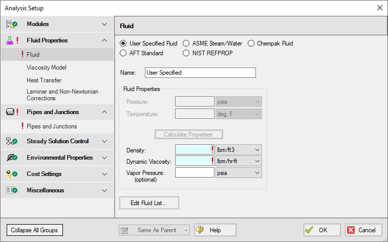
Figure 3: The Analysis Setup tracks the model’s status and allows users to specify required parameters
A. Define the Modules Group
Although Analysis Setup initially opens to the Fluid panel of the Fluid Properties group, the first group, Modules, always has a green check when you start AFT Fathom because there are no modules activated by default. No further input is required here.
B. Define the Fluid Properties Group
Next is the Fluid Properties group. This group allows you to specify your fluid properties (density, dynamic viscosity, and optional vapor pressure), viscosity model, heat transfer, and fluid corrections. Start by clicking on Fluid to open the Fluid panel (see Figure 4).
You can model the fluid properties in one of five ways.
-
User Specified Fluid: This fluid model allows you to directly type in the density, viscosity and vapor pressure. You cannot perform heat transfer analysis with a User Specified Fluid fluid.
-
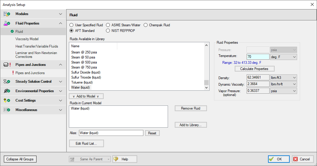
AFT Standard: This fluid model uses fluid data from the AFT Standard library. These fluid properties are either temperature dependent or dependent on the solids concentration. Type in the desired condition (e.g., temperature), click the Calculate Properties button and the required properties are calculated. Users can add their own fluids to this option. This model supports heat transfer analysis if specific heat and thermal conductivity data is included. Custom fluids are created by opening the Library Manager window from the Library menu or by clicking the Edit Fluid List button on the Fluid panel.
-
ASME Steam/Water: This fluid model obtains water data from the ASME Steam tables built into AFT Fathom. It also supports steam data, which can be used in AFT Fathom if incompressible.
-
NIST REFPROP: This fluid model allows you to select a single fluid or create a mixture of fluids from the REFPROP list. These fluid properties are pressure and temperature dependent, although some are temperature dependent only. This fluid model supports heat transfer analysis.
-
Chempak Fluid: This fluid model allows you to select a single fluid or create a mixture of fluids from the Chempak list. These fluid properties are pressure and temperature dependent, although some are temperature dependent only. This fluid model supports heat transfer analysis. Chempak is an optional add-on.
After selecting ASME Steam/Water, NIST REFPROP, or Chempak Fluid, you must then select a Fluid Phase: Liquid or Gas. Then, upon entering a pressure, AFT Fathom will display a temperature range applicable to liquid or gas, depending upon which was selected.
Note: Because heat transfer has a significant impact on compressible flow fluid properties and AFT Fathom calculates flow on an incompressible basis, heat transfer is disabled when Gas is selected as the Fluid Phase.
ØSelect AFT Standard, by clicking the radio button next to the name. Then choose Water (liquid) from the list and click Add to Model. The properties for AFT Standard water are given only as a function of temperature. Enter
ØCheck the groups on the left side of Analysis Setup and you should now see the second group is checked off.
On the Viscosity Model panel, users can specify how AFT Fathom will treat viscosity. By default, Newtonian is the viscosity model selected. AFT Fathom offers a variety of non-Newtonian models. However, for this example, the default selection of Newtonian will suffice.
On the Heat Transfer/Variable Fluids panel, users can specify variable fluid properties or enable heat transfer. For models with variable fluid properties, the values for density and viscosity are default fluid properties. You can then enter different property values, if desired, for any pipe in the Pipe Properties window. Fluids that allow heat transfer can be modeled by choosing the Heat Transfer with Energy Balance option. In this case, you will be required to also enter heat transfer information for the pipes and temperature for some of the junctions. By default, Constant Fluid Properties is selected and will suffice for this example.
On the Laminar and Non-Newtonian Corrections panel, users can specify the type of corrections that the solver will apply when flow is laminar or if a non-Newtonian viscosity model is selected. The default selections are applicable for most cases, so no input is required for this example.
C. Define the Pipes and Junctions Group
In order to fully define this group, there needs to be pipes and junctions on the Workspace. To lay out the classic three-reservoir model, you will place the three reservoir junctions and a branch junction on the Workspace. Then you will connect the junctions with pipes.
To go back to the Workspace and save the inputs made in Analysis Setup, click OK.
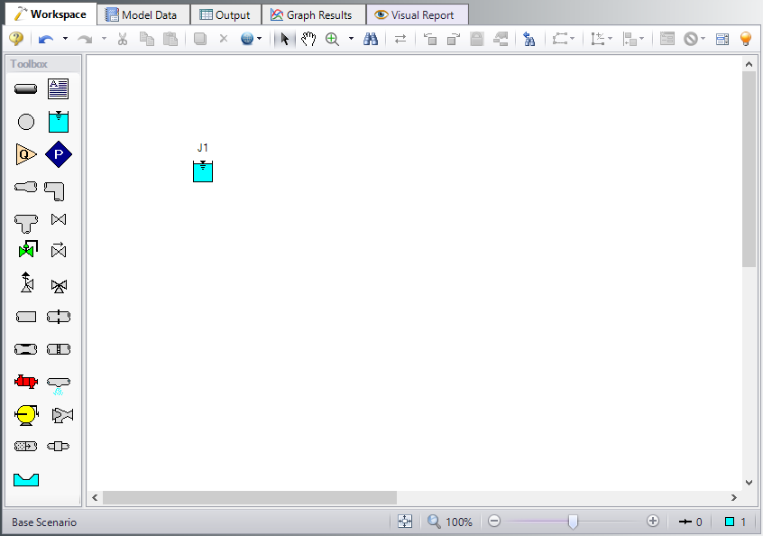
I. Place the first reservoir
ØTo start, drag a reservoir junction from the Toolbox and drop it on the Workspace. Figure 5 shows the Workspace with one reservoir.
Objects and ID numbers
Items placed on the Workspace are called objects. All objects are derived directly or indirectly from the Toolbox. AFT Fathom uses three types of objects: pipes, junctions, and annotations.
All pipe and junction objects on the Workspace have an associated ID number. For junctions, this number is, by default, placed directly above the junction and prefixed with the letter J. Pipe ID numbers are prefixed with the letter P. You can optionally choose to display either or both the ID number and the name of a pipe or junction. You also can drag the ID number/name text to a different location to improve visibility.
The reservoir you placed on the Workspace will take on the default ID number of 1. You can change this to any desired number greater than zero and up to 99,999.
Editing on the Workspace
Once on the Workspace, junction objects can be moved to new locations and edited with the features on the Edit menu. Cutting, copying, and pasting are all supported.
II. Place the second and third reservoirs
The remaining two reservoirs can be created the same way as the first one or they can be derived from the existing reservoir.
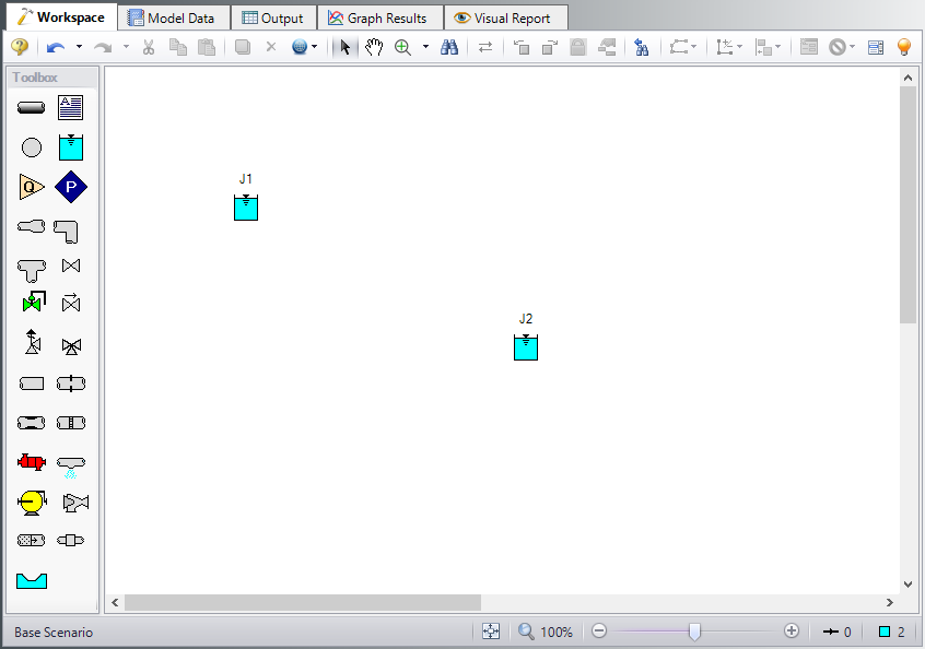
ØTo create a second reservoir from the existing one, select junction J1 by clicking it with the mouse. A red outline will surround the junction. Choose Duplicate from the Edit menu and move the J2 junction to the right of J1. Your Workspace should appear similar to that shown in Figure 6.
If you like, you can Undo the Duplicate operation and then Redo it to see how these editing features work. To undo an operation, click on the undo button on the Toolbar or choose Undo from the Edit menu. To redo an operation, choose Redo from the Edit menu.
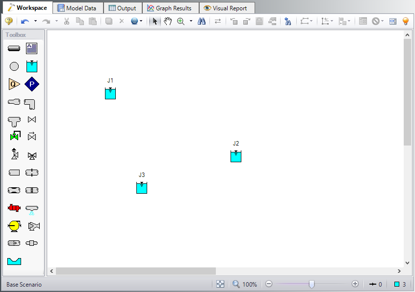
ØTo create the third junction, select one of the two reservoirs on the Workspace and once again choose Duplicate from the Edit menu. Arrange the three junctions, numbered J1, J2, and J3, as shown in Figure 7.
III. Place a branch junction
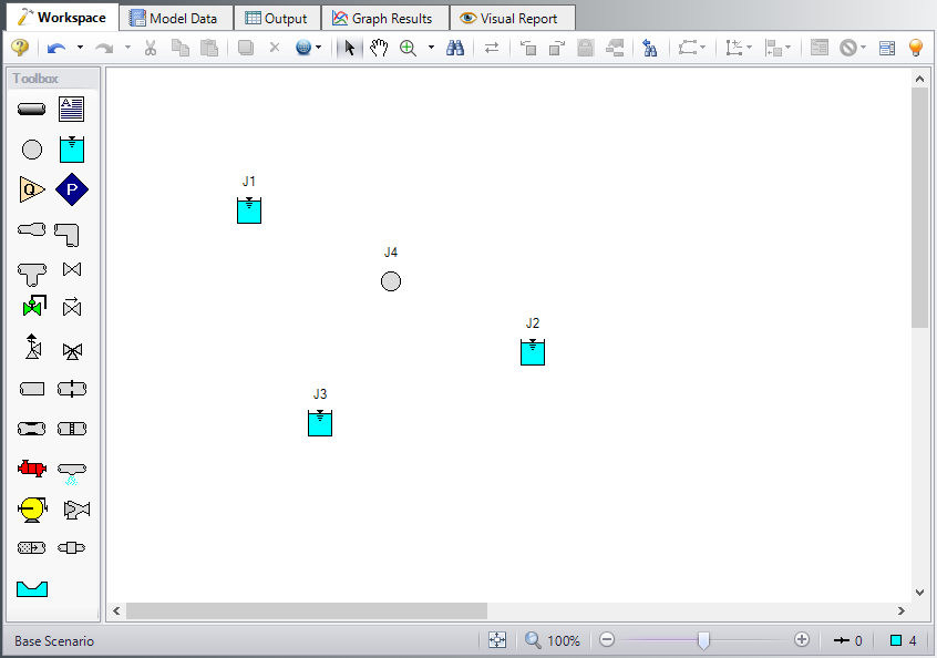
ØTo add a Branch junction, select a Branch from the Toolbox and place it on the Workspace as shown in Figure 8. The Branch will be assigned the default number J4.
Note: The relative location of objects in AFT Fathom is not important. Distances and heights are defined through dialog boxes. The relative locations on the Workspace establish the connectivity of the objects, but have no bearing on the actual length or elevation relationships.
ØBefore continuing, save the work you have done so far. Choose Save As from the File menu and enter a file name (Three Reservoir Problem, perhaps) and AFT Fathom will append the .fth extension to the file name.
IV. Draw a pipe between J1 and J4
Now that you have four junctions, you need to connect them with pipes.
ØTo create a pipe, click the Pipe Drawing tool icon. The pointer will change to a crosshair when you move it over the Workspace. Draw a pipe above the junctions, similar to that shown in Figure 9.
The pipe object on the Workspace has an ID number (P1) shown near the center of the pipe.
ØTo place the pipe between J1 and J4, use the mouse to grab the pipe in the center, drag it so that its left endpoint falls within the J1 Reservoir icon, then drop it there (see Figure 10). Next, grab the right endpoint of the pipe and stretch the pipe, dragging it until the endpoint terminates within the J4 Branch icon (see Figure 11).
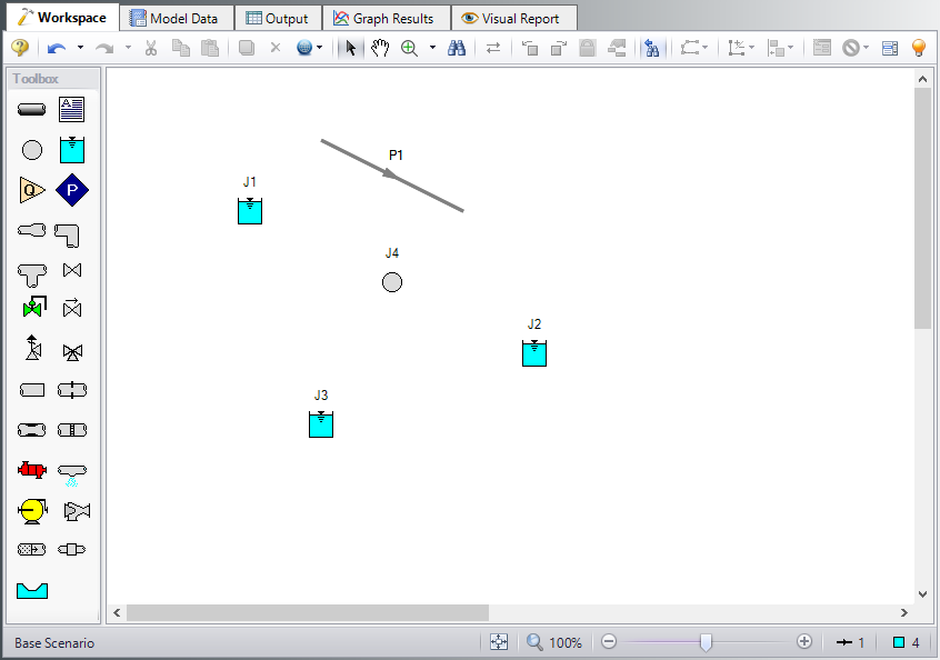
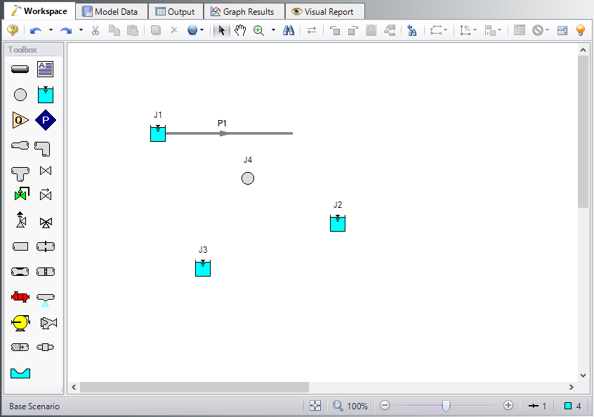
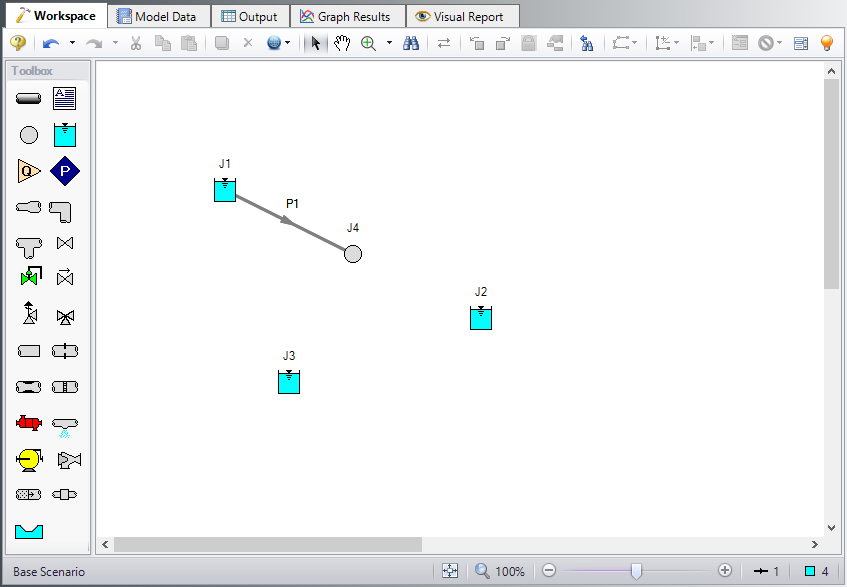
Figure 11: Three Reservoir Problem with first pipe connected
Reference positive flow direction
Located on the pipe is an arrow that indicates the reference positive flow direction for the pipe. AFT Fathom assigns a flow direction corresponding to the direction in which the pipe is drawn. You can reverse the reference positive flow direction by choosing Reverse Direction from the Arrange menu or selecting the reverse direction button on the Workspace Toolbar.
In general, the reference positive flow direction indicates which direction is considered positive. However, when used with pumps and certain other junction types the pipes must be in the correct flow direction because that is how AFT Fathom determines which side is suction and which is discharge. If the reference positive direction is the opposite of that obtained by the Solver, the output will show the flow rate as a negative number.
V. Add the remaining pipes
A faster way to add a pipe is to draw it directly between the desired junctions.
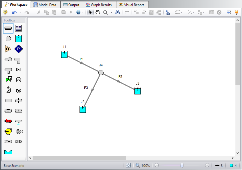
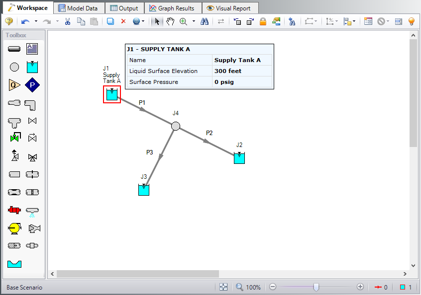
ØActivate the pipe drawing tool again (double-click to allow pipe drawing tool to stay active). Position the cursor on the J4 Branch. Press and hold the left mouse button. Stretch the pipe to the J2 Reservoir then release the mouse button. Then draw a third pipe from the J4 Branch to the J3 Reservoir. Your model should now look similar to Figure 12. In Figure 12, the J3 label has been moved slightly to the left (using drag-and-drop) so it is more visible.
At this point all the objects in the model are graphically connected. Save the model by selecting Save from the File menu or Toolbar.
Note: It is generally desirable to lock your objects to the Workspace once they have been placed. This prevents accidental movement and disruption of the connections. You can lock all the objects by choosing Select All from the Edit menu, then selecting Lock Object from the Arrange menu. The lock button on the Toolbar will appear depressed indicating it is in an enabled state, and will remain so as long as any selected object is locked. Alternatively, you can use the grid feature enabled from the Arrange menu or the User Options under the Tools menu bar and specify that the pipes and junctions snap to grid.
VI. Define the pipes and junctions
To fully define the Pipes and Junctions group in Analysis Setup, all pipes and junctions must be connected and have the proper input data.
Object status
Every pipe and junction has an object status. The object status tells you whether the object is defined according to AFT Fathom's requirements. To see the status of the objects in your model, click the floodlight icon on the Workspace Toolbar (alternatively, you could choose Show Object Status from the View menu). Each time you click the floodlight, Show Object Status is toggled on or off.
When Show Object Status is on, the ID numbers for all undefined pipes and junctions are displayed in red on the Workspace. Objects that are completely defined have their ID numbers displayed in black. (These colors are configurable through User Options from the Tools menu.)
Because you have not yet defined the pipes and junctions in this sample problem, all the objects' ID numbers will change to red when you turn on Show Object Status.
Undefined Objects window
The Undefined Objects window lists all undefined pipes and junctions and further displays the items that are not yet defined.
VII. Define Reservoir J1
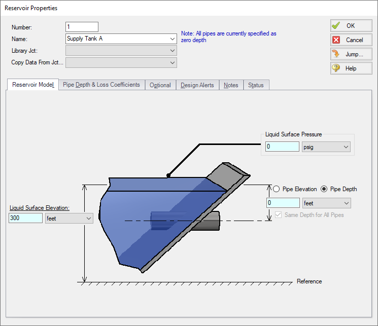
ØTo define the first reservoir, open the J1 Reservoir Properties window (see Figure 13) by double-clicking the J1 icon. Enter a reservoir Liquid Surface Elevation of
Note: You can also open an object's Properties window by selecting the object (clicking on it) and then either pressing the Enter key or clicking the Open Pipe/Jct Window icon on the Toolbar.
ØEnter a Liquid Surface Pressure of
Note: You can specify preferred units for many parameters (such as meters for length) in the User Options window.
You can give the object a name, if desired, by entering it in the Name field at the top of the window. In Figure 13, the name of this reservoir is Supply Tank A. By default the junction’s name is the junction type. The name can be displayed on the Workspace, Visual Report or in the Output.
Most junction types can be entered into a custom library allowing the junction to be used multiple times or shared between users. To select a junction from the custom library, choose the desired junction from the Library list. The current junction will get the properties from the library junction.
The Copy Data From Jct list will show all the junctions of the same type in the model. This will copy the selected parameters from an existing junction in the model to the current junction.
The pipe table on the Pipe Depth & Loss Coefficients tab allows you to specify entrance and exit loss factors for each pipe connected to the reservoir (in this case there is one). You can enter standard losses by selecting the option buttons at the right. The default selection is the Custom option with loss factors specified as zero. To later change the loss factors, click within the pipe table and enter the loss. You can also specify a depth for the pipe.
The Optional tab allows you to enter different types of optional data. You can select whether the junction number, name, or both are displayed on the Workspace. Some junction types also allow you to specify an initial pressure as well as other junction specific-data. The junction icon graphic can be changed, as can the size of the icon.
Design Alerts can be entered for most junctions, which are applied to the pressure loss calculations for the junction in order to give additional safety margin to the model.
Each junction has a tab for Notes, allowing you to enter text describing the junction or documenting any assumptions.
The Status tab will list undefined parameters of the junction.
The highlight feature displays all the required information in the Properties window in light blue as shown in Figure 13. The highlight is on by default. You can toggle the highlight off and on by double-clicking anywhere in the window or by pressing the F2 key. The highlight feature can also be turned on or off by selecting it on the User Options menu. For the remainder of the examples, we will keep the highlight feature turned off.
ØClick OK. If Show Object Status is turned on, you should see the J1 ID number turn black again, telling you that J1 is now completely defined.
The Inspection feature
You can check the input parameters for J1 quickly, in read-only fashion, by using the Inspection feature. Position the mouse pointer on J1 and hold down the right mouse button. An information box appears, as shown in Figure 14.
Inspecting is a faster way of examining the input in an object than opening the Properties window.
VIII. Define junctions J2, J3, and J4
-
J2 Reservoir
-
Liquid Surface Elevation = 200 feet
-
Liquid Surface Pressure = 0 psig
-
Pipe Depth = 0 feet (default)
-
-
J3 Reservoir
-
Liquid Surface Elevation = 100 feet
-
Liquid Surface Pressure = 0 psig
-
Pipe Depth = 0 feet (default)
-
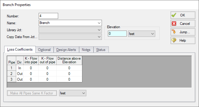
ØOpen the J4 Branch Properties window (see Figure 15). In this window, all three connecting pipes should be displayed in the pipe table area. You could associate loss factors with each pipe by clicking within the pipe table and entering the data.
ØEnter an elevation of zero
ØSave the model again before proceeding.
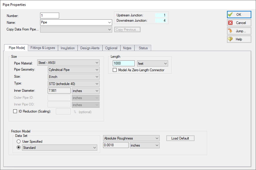
IX. Define Pipe P1
Data for pipes and junctions can be entered in any order. In this example, we did the junctions first. The next step is to define all the pipes. To open the Pipe Properties window, double-click the pipe object on the Workspace.
ØFirst open the Pipe Properties window for Pipe P1 (see Figure 16). For Pipe P1, enter a length of
The Pipe Properties window
The Pipe Properties window offers control over all important flow system parameters that are related to pipes.
The Inspect feature also works within the Pipe Properties window. To Inspect a connected junction, position the mouse pointer on the connected junction's ID number and hold down the right mouse button. This is helpful when you want to quickly check the properties of connecting objects. (You can also use this feature in junction Properties windows for checking connected pipe properties.)
By double-clicking the connected junction number, you can jump directly to the junction's Properties window. Or you can click the Jump button to jump to any other part of your model.
X. Define Pipes P2 and P3
Both pipes have a Pipe Material of Steel - ANSI, Size of 8 inch, and Type of STD (Schedule 40).
-
P2
-
Length = 2000 feet
-
-
P3
-
Length = 3000 feet
-
The Pipes and Junctions group should now be complete. Everything is ready to submit to the Solver.
ØBefore running the model, save it one more time. It is also a good idea to review the input using the Model Data window.
D. Define the remaining groups in Analysis Setup
Open Analysis Setup once more to confirm that all groups are defined. No inputs or alterations are required to complete the last three groups: Steady Solution Control, Environmental Properties, and Miscellaneous. All seven groups should have a green checkmark next to its name. Click OK.
D. Review input in the Model Data window
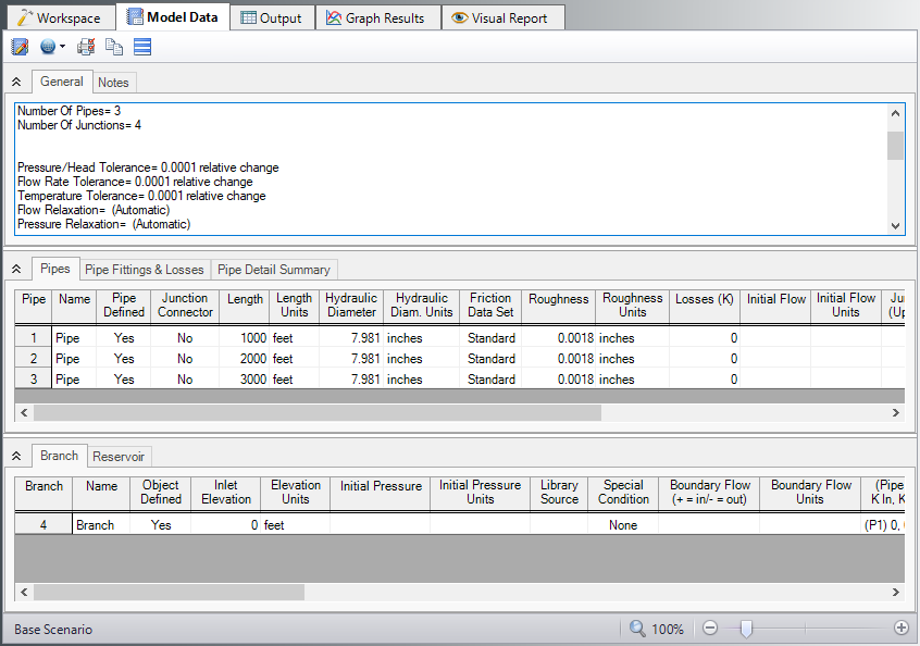
The Model Data window is shown in Figure 17. To change to this window, you can select it from the Primary Window tabs, Window menu, or pressing CTRL+M. The Model Data window gives you a text-based perspective of your model. Selections can be copied to the clipboard and transferred into other Windows programs, saved to a formatted file, printed to an Adobe PDF, or printed out for review.
Data is displayed in three general areas. The top is called the general area, the middle the pipe area and the bottom the junction area.
The Model Data window allows access to all Properties windows by double-clicking the appropriate ID number in the far left column of the table. You may want to try this right now.
Step 3. Run the Solver
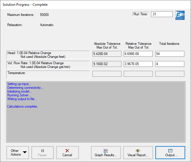
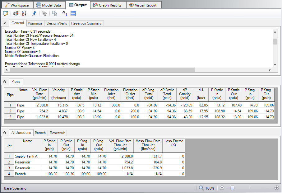
ØClick Run Model from the Toolbar or from the Analysis Menu. During execution, the Solution Progress window is displayed (see Figure 18). You can use this window to pause or cancel the Solver's activity. When the solution is complete, the Output, Visual Report, and Graphs Results windows can be accessed directly from the Solution Progress window. Click the Output button and the text-based Output window will appear (see Figure 19). The information in the Output window can be reviewed visually, saved to file, exported to a spreadsheet-ready format, copied to the clipboard, printed to an Adobe PDF file, and printed out on the printer.
Step 4. Review the output
The Output window is similar in structure to the Model Data window. Three areas are shown, and you can minimize or enlarge each area by clicking the arrow next to the General, Pipes, and Junctions tabs or from the View menu.
A. Specify output control
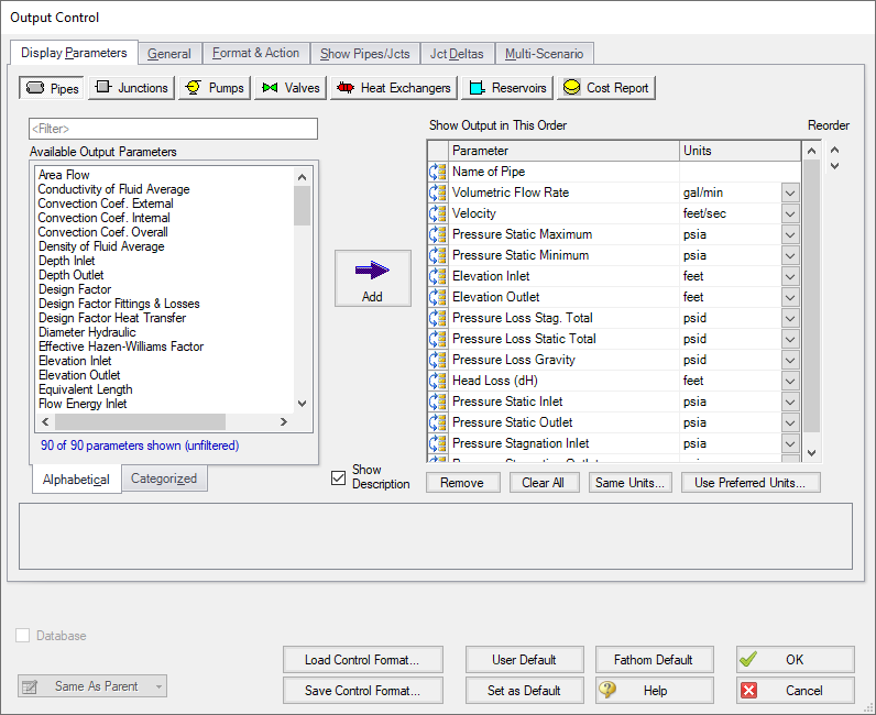
By default, AFT Fathom has a predefined set of Output Control parameters that are specified and the default units used depend on which unit set was selected when first running AFT Fathom (see Figure 1). A default title is also assigned in the Output Control.
ØOpen Output Control from the Tools menu (Figure 20). Click the General tab, enter a new title (if you like you can title this Classic Three-Reservoir Problem), then click OK to accept the title and other default data.
In addition, this window allows you to select the specific output parameters you want in your output. You also can choose the units for the output.
B. Modify the output format
If you selected the default AFT Fathom Output Control, the Pipe Results table will show volumetric flow rate in the second column (Figure 19) with units of
-
Select Output Control from the Tools menu or Toolbar. On the right side of the Pipe tab is the list of selected output parameters. Click Volumetric Flow Rate and change the units by selecting
-
Click OK to display changes to the current results. You should see the volumetric flow rate results, still in the second column, in units of
-
Select Output Control from the Tools menu one more time. The reorder icons on the left side of the Output List allows you to reorder parameters in the list.
-
Select the Velocity parameter and use the Reorder scroll bar to move it up to the top of the parameter list.
-
Click OK to display the changes to the current results. You will see in the Pipe Results table that the first column now contains Velocity and the third column contains the volumetric flow rate. The Output Control window allows you to obtain the parameters, units and order you prefer in your output. This flexibility will help you work with AFT Fathom in the way that is most meaningful to you, reducing the possibility of errors.
-
Lastly, double-click the column header Velocity in the Output window Pipe Results Table. This will open a window in which you can change the units again if you prefer. These changes are extended to the Output Control parameter data you have previously set.
C. View the Visual Report
-
Change to the Visual Report window by choosing it from the Window menu, clicking on the Visual Report tab on the tool bar, or by pressing CTRL+I. This window allows you to integrate your text results with the graphic layout of your pipe network.
-
The Visual Report Control window should open immediately, shown in Figure 21. Select Volumetric Flow Rate in the Pipe Output area and Pressure Static Inlet in the Common Junction Output area. Click Show at the bottom. The Visual Report window graphic is generated (see Figure 22).
It is common for the text in the Visual Report window to overlap when first generated. You can change this by selecting smaller fonts or by dragging the text to a new area to increase clarity (this has already been done in Figure 22). This window can be printed or copied to the clipboard for import into other Windows graphics programs, saved to a file, or printed to an Adobe PDF file.
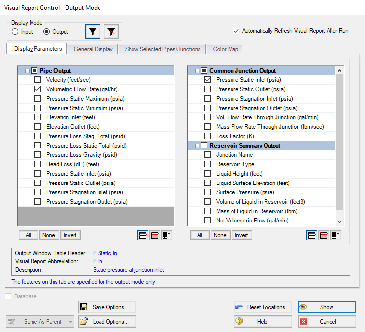
Figure 21: The Visual Report Control window selects content for the Visual Report window, which integrates results with model layout
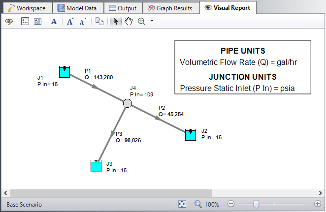
Figure 22: The Visual Report window displays output data on the input schematic. It also can operate in Input Mode where it displays input data
D. Graph the results
ØChange to the Graph Results window by clicking the Graph Results tab. The Graph Results window offers full-featured Windows plot preparation.
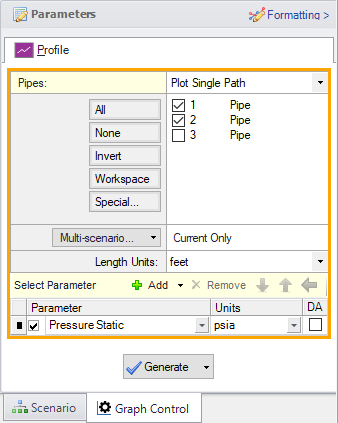
The Graph Parameters menu will automatically be displayed in the Quick Access Panel on the far right of the Graph Results Window and is where you are to specify which graphs to generate.
The Profile graph tab in the Graph Parameters menu will also be selected by default on Quick Access Panel. Make sure the Plot Single Path option is selected from the Pipes drop-down menu. Select pipes 1 and 2 from the pipes list. Choose Pressure Static from the Parameter drop-down menu. Make sure
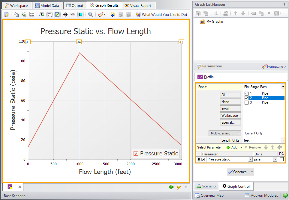
A graph appears showing the static pressure along the flow-path defined by pipes 1 and 2 in Figure 24.
You can use the other buttons in the Graph Results window to change the graph appearance and to save and import data for cross-plotting. The Graph Results window can be printed, saved to file, copied to the clipboard, or printed to an Adobe PDF file. The graph’s x-y data can be exported to file or copied to the clipboard.
Note that the graph guide, located at the top right of the Graph Results window and represented with the What Would You Like to Do? icon, can guide you through the development of your graph. This feature can be hidden by clicking on the icon.
Conclusion
You have now used AFT Fathom's five Primary Windows to build a simple model. Review the rest of the Fathom Help File contents for more detailed information on each of the windows and functions.


