Cost Calculation - Beginner (Metric Units)
Controlled Heat Exchanger Temperature (English Units)
Summary
This example demonstrates how to set up cost calculations in AFT Fathom.
Determine the cost of the heat exchanger system over a 10-year period including material, installation, and energy costs.
Topics Covered
-
Estimating simple costs
-
Connecting cost libraries
-
Using Cost Settings
-
Using the Cost Report
Required Knowledge
This example assumes the user has already worked through the Beginner: Three Reservoir Problem example, or has a level of knowledge consistent with that topic. You can also watch the AFT Fathom Quick Start Video Tutorial Series on the AFT website, as it covers the majority of the topics discussed in the Three-Reservoir Problem example.
Model Files
This example uses the following files, which are installed in the Examples folder as part of the AFT Fathom installation:
-
Controlled HX Temperature.dat - engineering library
-
Controlled HX Temperature - Junction Costs.cst - cost library for Controlled HX Temperature.dat
-
Controlled HX Temperature - Pipe Costs.cst - cost library for Steel - ANSI
Step 1. Start AFT Fathom
From the Start Menu choose the AFT Fathom 12 folder and select AFT Fathom 12.
To ensure that your results are the same as those presented in this documentation, this example should be run using all default AFT Fathom settings, unless you are specifically instructed to do otherwise.
If you have already worked the Controlled Heat Exchanger Temperature example for either the GSC or XTS modules, you can open the file you built for those examples, create a new scenario for this example, and then skip to Step 4.
Important: The XTS and GSC modules and cost calculations can be performed in the same run to simulate control functions over time, but we are not going to do this here. Before proceeding, make sure to disable GSC by selecting the radio button for Ignore under GSC in the Modules panel in Analysis Setup. Also, make sure to disable XTS by selecting Steady Only in the XTS section.
Step 2. Define the Fluid Properties Group
-
Open Analysis Setup from the toolbar or from the Analysis menu.
-
Open the Fluid panel then define the fluid:
-
Fluid Library = AFT Standard
-
Fluid = Water (liquid)
-
After selecting, click Add to Model
-
-
Temperature = 21 deg. C
-
-
This calculates the default fluid properties to use in the model to initialize the heat transfer calculations.
-
Open the Heat Transfer/Variable Fluidspanel:
-
Heat Transfer = Heat Transfer With Energy Balance (Single Fluid)
-
Step 3. Define the Pipes and Junctions Group
At this point, the first two groups are completed in Analysis Setup. The next undefined group is the Pipes and Junctions group. To define this group, the model needs to be assembled with all pipes and junctions fully defined. Click OK to save and exit Analysis Setup then assemble the model on the workspace as shown in the figure below.
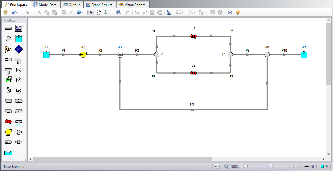
Pipe Properties
-
All Pipes
-
Pipe Material = Steel - ANSI
-
Pipe Geometry = Cylindrical Pipe
-
Size = 8 inch
-
Type = STD (schedule 40)
-
Friction Model Data Set = Standard
-
Length =
| Pipe | Length (meters) |
|---|---|
|
1 & 3-8 |
6 |
| 2 | 1.5 |
| 9 | 60 |
| 10 | 30 |
Junction Properties
-
J1 & J9 Reservoirs
-
Liquid Surface Elevation = 6 meters
-
Liquid Temperature = 90 deg. C
-
Update Density with Temperature = Checked
-
Liquid Surface Pressure = 0.3 barG (30 kPa (g))
-
Pipe Depth = 0 meters
-
-
J2 Pump
-
Inlet Elevation = 0 meters
-
Pump Model = Centrifugal (Rotodynamic)
-
Analysis Type = Pump Curve
-
Enter Curve Data =
-
| Volumetric | Head |
|---|---|
| m3/hr | meters |
| 0 | 20 |
| 115 | 18 |
| 230 | 12 |
-
Curve Fit Order = 2
-
J3 Three Way Valve
-
Elevation = 0 meters
-
Combined Flow = P2
-
Split Flow Pipe #1 = P3
-
Split Flow Pipe #2 = P9
-
Loss Model = Cv
-
Open Percentage Data =
-
| Open Pct. | Cv Pipe #1 | Cv Pipe #2 |
|---|---|---|
| 0 | 0 | 100 |
| 100 | 100 | 0 |
-
Actual Percent Open = 75%
-
J4, J7, & J8 Branch Junctions
-
Elevation = 0 meters
-
-
J5 & J6 Heat Exchangers
-
Inlet Elevation = 0 meters
-
Loss Model tab
-
Loss Model = K Factor
-
K = 1400
-
-
Thermal Data tab
-
Thermal Model = Counter-Flow
-
Heat Transfer Area = 148 m2
-
Overall Heat Transfer Coefficient = 280 W/m2-K
-
Flow Rate = 90 kg/sec
-
Specific Heat = 4.2 kJ/kg-K
-
Inlet Temperature = 4.5 deg. C
-
-
ØTurn on Show Object Status from the View menu to verify if all data is entered. If so, the Pipes and Junctions group in Analysis Setup will have a check mark. If not, the uncompleted pipes or junctions will have their number shown in red. If this happens, go back to the uncompleted pipes or junctions and enter the missing data.
Step 4. Define the Cost Settings group
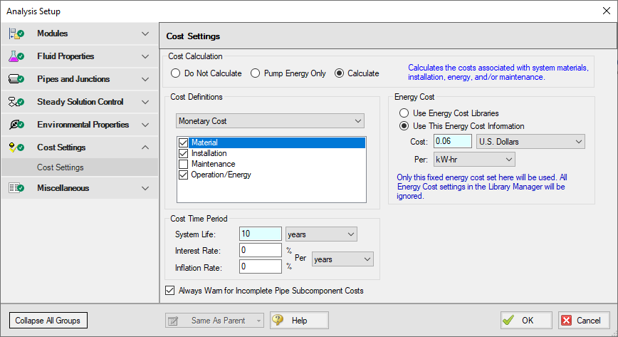
To perform cost calculations they will first need to be enabled. Do this by opening Analysis Setup, navigating to the Cost Settings panel , then selecting Calculate in the Cost Calculation section. If it is only desired to estimate energy costs, the Pump Energy Only option could be selected instead to simplify the input.
The Cost Settings panel is where the types of costs to be included in the cost calculations are specified. The Cost Settings panel is shown in Figure 2.
The Cost Definitions section allows you to specify the type of costs to be determined. You may select from engineering parameter costs, such as pipe weight, or actual monetary costs, including material and installation costs. For this example, select Monetary Costs, if not already selected. Include Material, Installation, and Operation/Energy costs by selecting them from the list of available monetary costs, as shown in Figure 2.
Energy cost data can be specified through an energy cost library, or by directly entering an energy cost on the Cost Settings panel. Using an energy cost library allows you to specify multiple energy costs, such as energy costs at both peak and off-peak rates. For this example, select Use This Energy Cost Information and enter a Cost of 0.06 U.S. Dollars Per kW-hr, as shown in Figure 2.
The system lifetime to be applied for the cost calculations is specified in the Cost Time Period section. You can also specify interest and inflation rates to be applied to the cost calculations as well. For this example, enter a system life of 10 years, as shown in Figure 2, then close the Cost Settings panel by clicking the OK button.
Step 5. Engineering and Cost Libraries
The actual material and installation costs that would be used with cost calculations are contained in cost libraries. The cost libraries needed for this example already exist, and just need to be accessed.
The Library Manager (opened from the Library menu) shows all of the available and connected libraries. Libraries can either be engineering libraries or cost libraries. Cost libraries are always associated with an engineering library, and are thus displayed subordinate to an engineering library in the library lists.
Here we will summarize some key aspects of libraries:
-
Cost information for a pipe is accessed from a cost library. Cost library items are based on corresponding items in an engineering library. (The engineering library also includes engineering information such as pipe diameters, hydraulic loss factors, etc.)
-
To access a cost for a particular pipe or junction in a model, that pipe or junction must be based on items in an engineering library that is connected to the model file.
-
There can be multiple cost libraries associated with and connected to an engineering library (such as regionally varying costs, or multiple foreign currencies). This makes it easier to manage costs of items.
Open the Library menu and select Library Manager. Click Add Existing Library, select the Controlled HX Temperature.dat engineering library from the AFT Fathom 12 Examples folder, and click Open. The engineering library titled Controlled HX Temperature should now appear in the list of available libraries.
Now add the cost libraries by clicking Add Existing Cost Library, and browsing to the Controlled HX Temperature - Junction Costs.cst and the Controlled HX Temperature - Pipe Costs.cst cost library files.
These libraries should connect automatically. If not, connect the newly added engineering and cost libraries by checking the box next to the name in the list of available libraries.
The Library Manager should appear as shown in Figure 3. The Library Manager window displays all of the available and connected libraries.
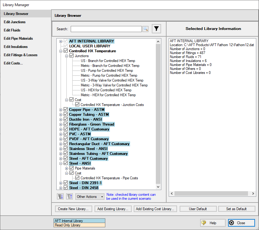
The engineering libraries associated with these two cost libraries are the Steel - ANSI pipe material library, and an external library called Controlled HX Temperature. For the cost data in the two cost libraries to be accessed by pipes and junctions in the model, the pipes and junctions must use these two engineering libraries.
The pipes for this example are already using data from the Steel - ANSI pipe material library, so no modifications need to be made for the pipes. All of the junctions except the reservoir junctions must be modified to use the junction data contained in the engineering libraries. Do this by opening the properties window for each junction, and selecting the junction name displayed in the Library list, as shown in Figure 4 for the Three-Way Valve Junction.
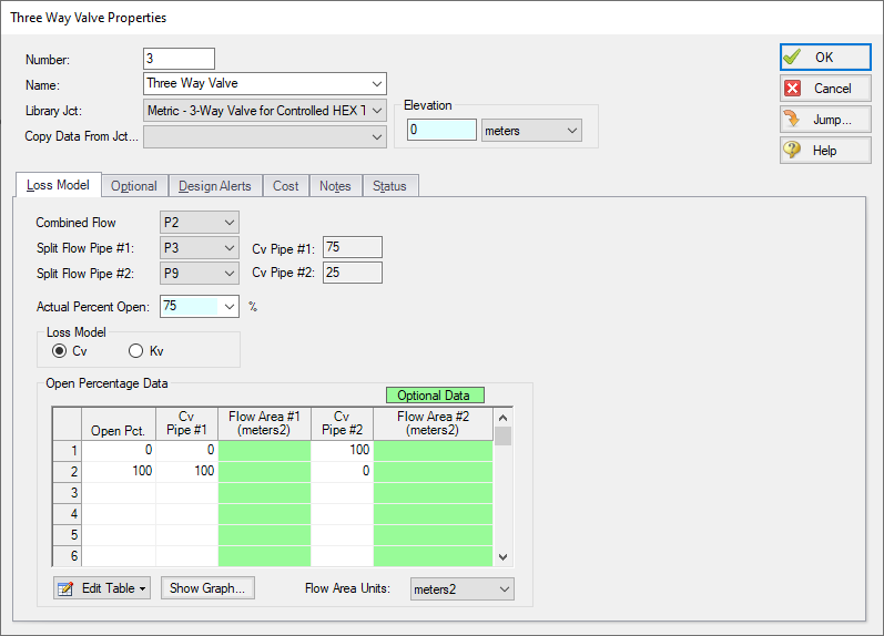
Figure 4: The junctions to be included in the cost analysis must be associated with an engineering library
Step 6. Including objects in the Cost Report
The final step before performing a cost analysis is to specify which pipes and junctions you want to be included in the final cost report. This is done by opening the properties window, navigating to the Cost tab, and choosing Include in Cost Report for each pipe and junction to be included, as shown for Pipe 1 in Figure 5.
The Global Edit feature may be used to update this information for all of the pipes and junctions.
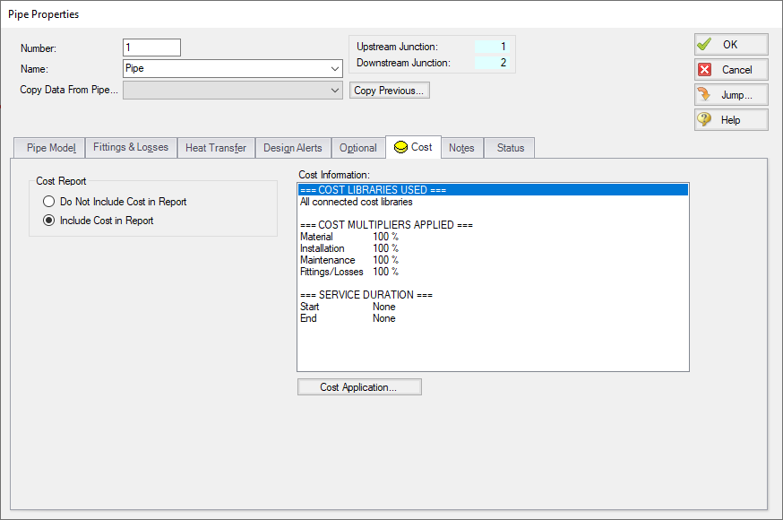
Figure 5: The Cost tab on the pipe and junction Properties windows is used to include the objects in the Cost Report
Step 7. Run the Model
Click Run Model on the toolbar or from the Analysis menu. This will open the Solution Progress window. This window allows you to watch as the AFT Fathom solver converges on the answer. This model runs very quickly. Now view the results by clicking the Output button at the bottom of the Solution Progress window.
Step 8. Examine the Cost Report
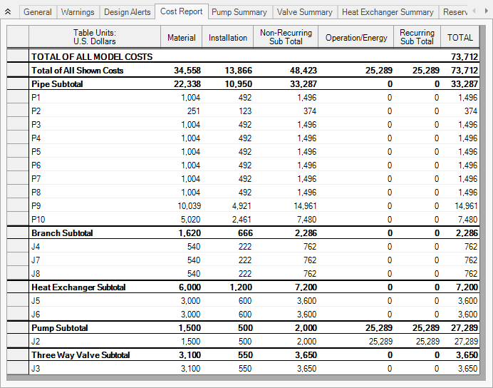
The Cost Report is displayed in the General Results section of the Output Window. View the Cost report by selecting the Cost Report Tab. The content of the Cost Report can be controlled from the Output Control window. Figure 6 shows the Cost Report for this example with the Material, Installation, Energy, and Total costs displayed.
The Cost Report shows the total system cost, as well as the individual totals for the material, installation, and energy costs. In addition, the Cost Report displays the detailed cost for each pipe, junction, and fitting that was included in the report. The items are grouped together by type, and a subtotal for each category is listed.
Cost Analysis Summary
The cost analysis for this example shows the total system cost over 10 years for the heat exchanger system is