Beginner: Heat Transfer in a Pipe - GSC (English Units)

Summary

The objective of this example is to demonstrate how goals and variables are used in the GSC module to achieve an objective.

For this example, we will use the GSC module to determine the flow rate required such that the fluid at the outlet of a 30-meter section of pipe, with heat transfer, reaches a temperature of 50 deg. C.

Note: This example can only be run if you have a license for the GSC module.

Topics Covered

• Defining the Goal Seek and Control group

• Understanding Goal Seek and Control Output

Required Knowledge

This example assumes the user has already worked through the Walk-Through Examples section, and has a level of knowledge consistent with the topics covered there. If this is not the case, please review the Walk-Through Examples, beginning with the Beginner: Three Reservoir Model example. You can also watch the AFT Fathom Quick Start Video Tutorial Series on the AFT website, as it covers the majority of the topics discussed in the Three-Reservoir Model example.

Model Files

This example uses the following files, which are installed in the Examples folder as part of the AFT Fathom installation:

• Metric - Heat Transfer.fth

• Metric - Heat Transfer - GSC.fth

Step 1. Start AFT Fathom

From the Start Menu choose the AFT Fathom 12 folder and select AFT Fathom 12.

To ensure that your results are the same as those presented in this documentation, this example should be run using all default AFT Fathom settings, unless you are specifically instructed to do otherwise.

Step 2. Open the model

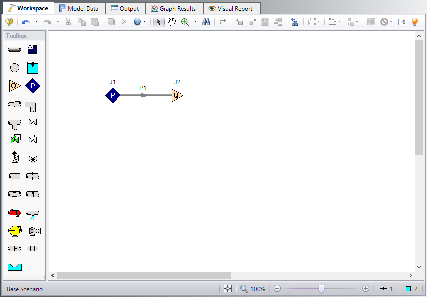
Open the Metric - Heat Transfer.fth example file listed above, which is located in the Examples folder in the AFT Fathom application folder. Save the file to a different folder. The workspace should look like Figure 1 below:

Step 3. Define the Modules group

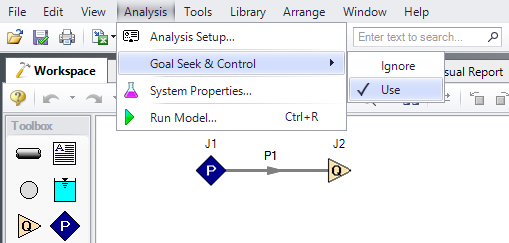
The GSC module is controlled through the Goal Seek and Control group in Analysis Setup. Open Analysis Setup, which should bring you to the Modules panel. Check the box next to Activate GSC. The Use option should automatically be selected, making GSC enabled for use. Alternatively, GSC can be enabled from the Analysis menu by going to the Goal Seek & Control option and selecting Use, as shown in Figure 2.

Step 4. Define the Goal Seek and Control Group

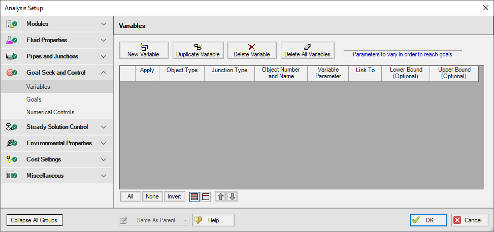
The Goal Seek and Control group is made up of three items: Variables, Goals, and Numerical Controls. The default settings in Numerical Controls will suffice for most applications and no input is necessary in this panel for this example. The variables and goals are defined in their respective panels. The Variables panel is shown in Figure 3 below:

Variables Panel

In the GSC module, variables are the parameters that the solver will modify in order to achieve the specified goals. There should be one variable defined for each goal.

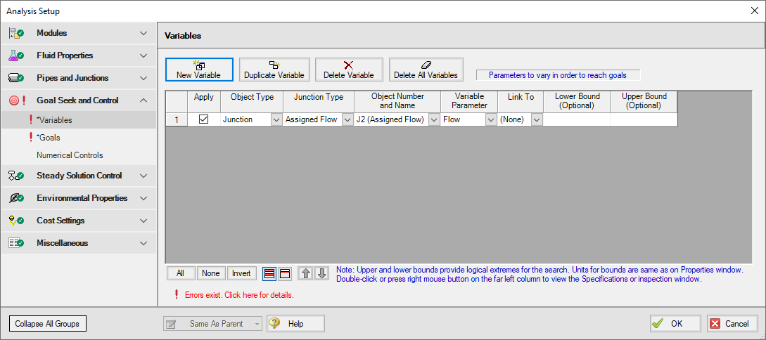
Open the Variables panel in the Goal Seek and Control group in Analysis Setup. The Variables panel allows you to create and modify the system variables. The object type and junction type are selected, then the name and number of the object to which the variable applies, and the object parameter that is to be varied are specified all on the Variables panel.

Do the following:

1. Click New Variable

2. Apply = Checked

3. Object Type = Junction

4. Junction Type = Assigned Flow

5. Junction Number and Name = J2 (Assigned Flow)

6. Variable Parameter = Flow

7. Link To = (None)

The Apply column allows users to specify which of the variables that have been defined will be used. This allows the flexibility of creating multiple variable cases, while only applying selected variables for any given run.

The Link To column allows users to apply the same variable to multiple objects. This allows users to force parameters for several objects to be varied identically.

Upper and Lower Bounds provide logical extremes during the goal search. For this case, leave both the lower bound and the upper bound values blank.

After entering the data, the Variables panel should appear as shown in Figure 4:

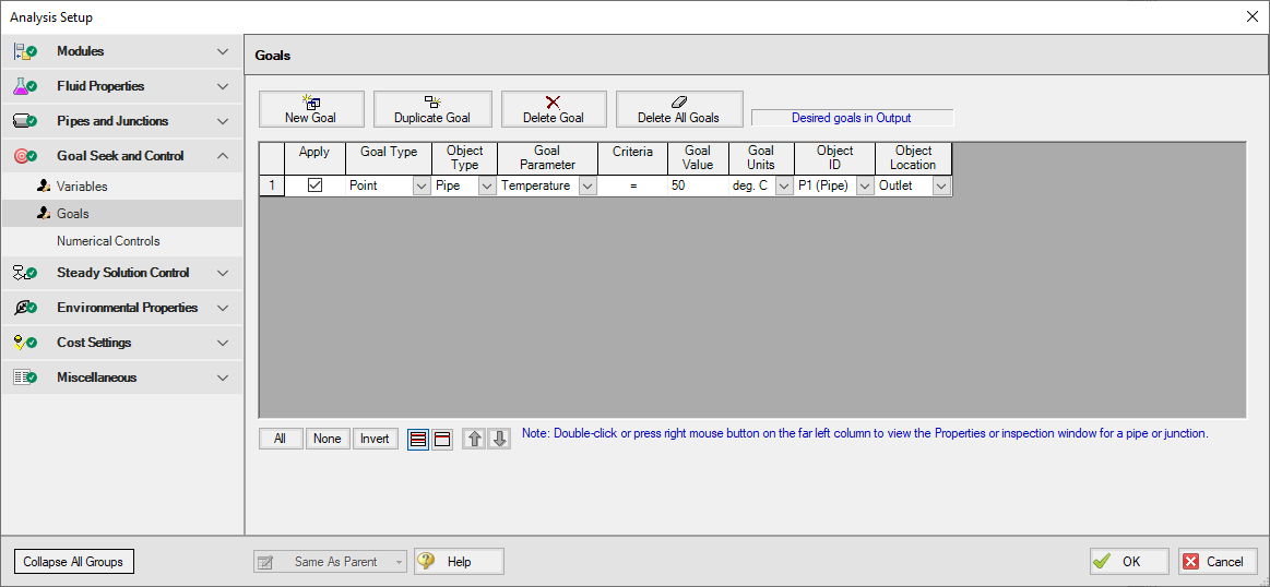
Goals Panel

Goals are the parameter values set by the user that Fathom adjusts the variables to achieve. There should be one goal defined for each variable.

Open the Goals panel in the Goal Seek and Control group. The Goals panel allows you to create and modify the system goals. The goal type, object type, and the goal parameter are selected. A criterion for determining if the goal has been met is then specified, along with a value and units for the goal parameter. You can select the object to which the goal applies, and, if applicable, the location on the object at which the goal applies (i.e. the inlet or outlet of a pipe object).

Do the following:

1. Click New Goal

2. Apply = Checked

3. Goal Type = Point

4. Object Type = Pipe

5. Goal Parameter = Temperature

6. Criteria = =

7. Goal Value = 50

8. Goal Units = deg. C

9. Object ID = P1 (Pipe)

10. Object Location = Outlet

After entering the data, the Goals panel should appear as shown in Figure 5:

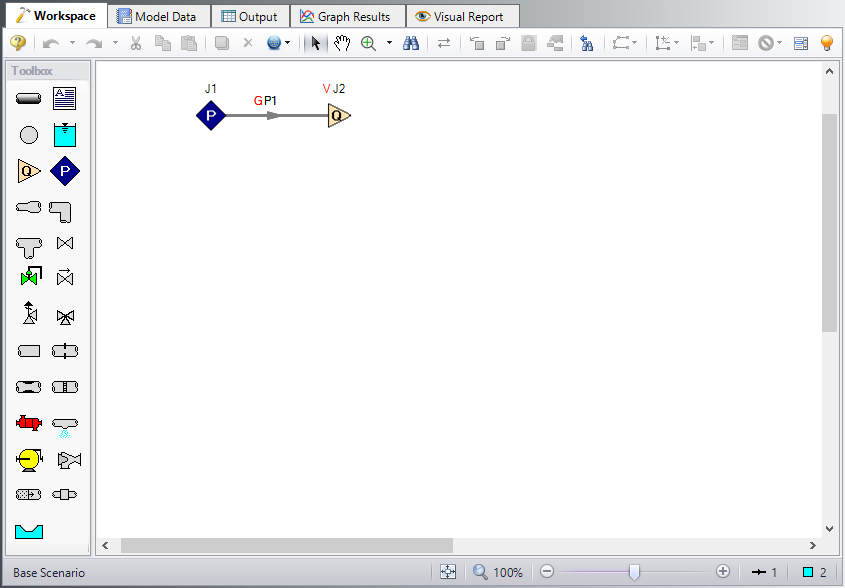
As variables and goals are added to a model, Fathom will display symbols beside the pipes and junctions that have variables or goals applied to them. The default is a V for variables, and a G for goals. The goal symbol is not displayed next to objects that are part of a group goal. This is illustrated in Figure 6:

Step 5. Run the Model

Click Run Model on the toolbar or from the Analysis menu. This will open the Solution Progress window. This window allows you to watch as the AFT Fathom solver converges on the answer. This model runs very quickly. Now view the results by clicking the Output button at the bottom of the Solution Progress window.

Step 6. Examine the Output

Figure 7 shows the Output window with the General, Pipes, and Junctions sections displayed.

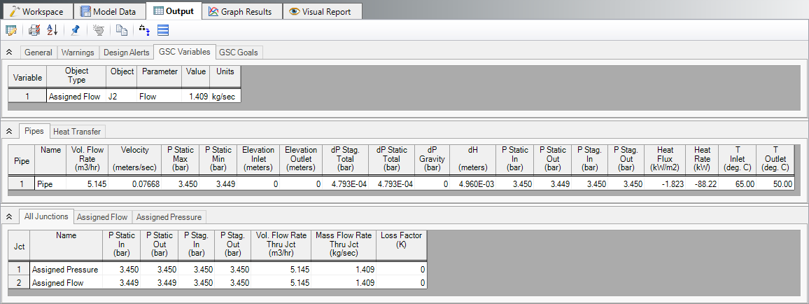
Figure 7: The Output window contains all the data that was specified in the output control window

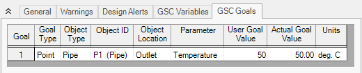
The results of the GSC analysis are shown in the General Output section in the GSC Variables and GSC Goals tabs. The GSC Variables tab shows the final value for the variable parameter, as shown in Figure 8. The GSC Goals tab shows the final value achieved for the goal, as shown in Figure 9.

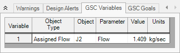
The GSC module analysis determined that a mass flow rate of 1.409 kg/sec (5.145 m3/hr) results in a pipe outlet temperature of 50 deg. C. In order to achieve the desired temperature, the assigned flow rate was varied from the initial value of 4.5 kg/s, to the final value of 1.409 kg/sec. In addition to the GSC module tabs in the General Output section, the resulting pipe flow and temperature results can be seen in the Pipes section of the Output Window.