Slurry System Feasibility Study - SSL (Metric Only)
Summary
Note: Because this example is presented in SI units in the reference from which it was taken, it is presented in the same units here for consistency when discussing the results.
This example demonstrates how the Settling Slurry (SSL) add-on module can be used to evaluate the feasibility of a slurry system operating point. The example is based on Case Study 13.1 found on page 329 of Slurry Transport Using Centrifugal Pumps, 3rd Edition, by Wilson, Addie, Sellgren, and Clift. Here only the 0.65 m case is evaluated.
An operating condition from a previous case study was selected:
Condition A:
D = 0.65 meters
Vsm = 4.84 meters/sec
Cvd = 0.20
Vm = 6.30 meters/sec
It was noted in the previous study that increasing Cvd and decreasing Vm reduced the specific energy consumption, and a revised operating point was also selected:
Condition B:
D = 0.65 meters
Vsm = 4.84 meters/sec
Cvd = 0.221
Vm = 5.70 meters/sec
Using these two operating points, determine whether either operating point would be feasible for the system.
Note: This example can only be run if you have a license for the SSL module.
Topics Covered
-
Entering solids data
-
Reviewing calculated slurry output
-
Evaluating stability of system operability
Required Knowledge
This example assumes the user has already worked through the Walk-Through Examples section, and has a level of knowledge consistent with the topics covered there. If this is not the case, please review the Walk-Through Examples, beginning with the Beginner: Three Reservoir Model example. You can also watch the AFT Fathom Quick Start Video Tutorial Series on the AFT website, as it covers the majority of the topics discussed in the Three-Reservoir Model example.
In addition the user should have worked through Pump Sizing for Sand Transfer System - SSL example.
Model Files
This example uses the following files, which are installed in the Examples folder as part of the AFT Fathom installation:
Step 1. Start AFT Fathom
From the Start Menu choose the AFT Fathom 12 folder and select AFT Fathom 12.
To ensure that your results are the same as those presented in this documentation, this example should be run using all default AFT Fathom settings, unless you are specifically instructed to do otherwise.
Step 2. Define the Modules Panel
Open Analysis Setup from the toolbar or from the Analysis menu. Navigate to the Modules panel. For this example, check the box next to Activate SSL and select Settling to enable the SSL module for use. The items in the Fluid Properties group will change to accommodate slurry definitions. Click OK to save the changes and exit Analysis Setup. Open the Analysis menu to see the new option called Slurry. From here you can quickly toggle between Disable mode (normal AFT Fathom) and Settling (SSL mode).
Step 3. Define the Fluid Properties Group
Open Analysis Setup from the toolbar or from the Analysis menu and input the following on the respective panels.
-
Carrier Fluid - Figure 1
-
Fluid Model = Basic (Water)
-
Temperature = 4 deg. C
-
-
Solids Definition - Figure 2
-
Slurry Calculation Method = Detailed
-
Solids Specifications = User Specified Solids Added
-
M (Stratification Ratio Exponent) = Calculated
-
Terminal Velocity Parameter = Vt / Vts (Xi)
-
Value = 0.56
-
Density = 2.65 S.G. water
-
d50 = 0.7 mm
-
d85 = 1 mm
-
-
Slurry Definition - Figure 3
-
Slurry Calculation Method = Detailed (this selection will be the same as on the Solids Definition panel)
-
Concentration Type = Volume Fraction
-
Amount Solids Added = 20 Percent
-
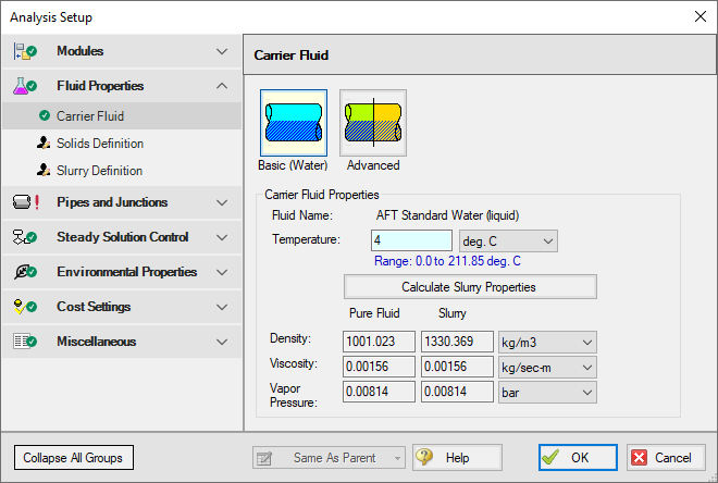
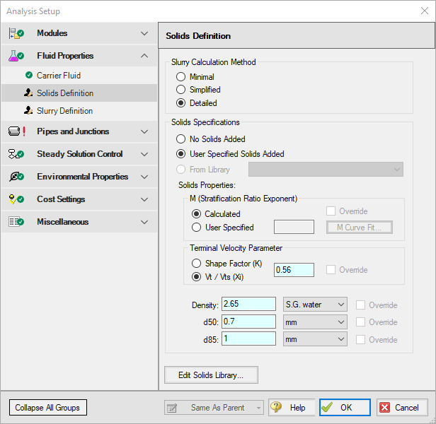
Figure 2: Solids Definition panel in the Fluid Properties group in Analysis Setup with SSL activated
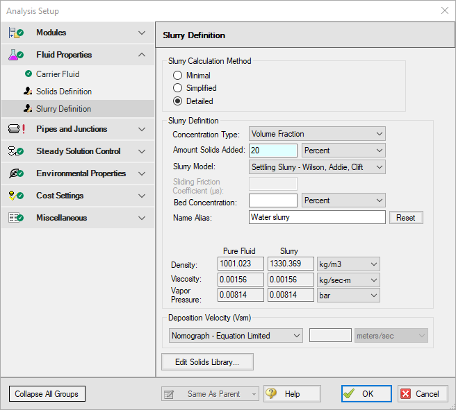
Figure 3: Slurry Definition panel in the Fluid Properties group in Analysis Setup with SSL activated
Step 4. Define the Pipes and Junctions Group
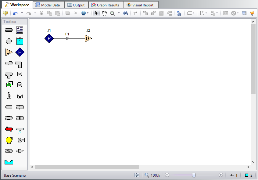
At this point, the first two groups are completed in Analysis Setup. The next undefined group is the Pipes and Junctions group. To define this group, the model needs to be assembled with all pipes and junctions fully defined. Click OK to save and exit Analysis Setup then assemble the model on the workspace as shown in the figure below.
Enter the following pipe and junction properties.
Pipe Properties
-
All Pipes
-
Pipe Material = (User Specified)
-
Pipe Geometry = Cylindrical Pipe
-
Inner Diameter = 0.65 meters
-
Friction Model Data Set = User Specified
-
Friction Factor = Explicit Friction Factor
-
Value = 0.012
-
Length = 100 meters
Junction Properties
-
J1 Assigned Pressure
-
Elevation = 0 meters
-
Pressure = 1 MPa
-
Pressure Specification = Stagnation
-
-
J2 Assigned Flow
-
Elevation = 0 meters
-
Type = Outflow
-
Flow Specification = Mass Flow Rate
-
Flow Rate = 4000 m-ton/hr Solids (metric tons equivalent to 4.0 x 10^6 kg/hr)
-
(metric tons equivalent to 4.0 x 10^6 kg/hr)
-
-
ØTurn on Show Object Status from the View menu to verify if all data is entered. If so, the Pipes and Junctions group in Analysis Setup will have a check mark. If not, the uncompleted pipes or junctions will have their number shown in red. If this happens, go back to the uncompleted pipes or junctions and enter the missing data.
Step 5. Run the Model
Click Run Model on the toolbar or from the Analysis menu. This will open the Solution Progress window. This window allows you to watch as the AFT Fathom solver converges on the answer. This model runs very quickly. Now view the results by clicking the Output button at the bottom of the Solution Progress window.
Step 6. Examine the Output
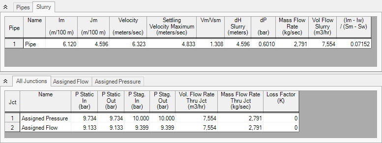
The maximum settling velocity for Condition A calculated by Fathom is 4.833 meters/sec, as shown in Figure 5. The value for the maximum settling velocity for Condition B can be reproduced in a similar fashion using Fathom.
Step 7. Evaluate System Operability
To determine the feasibility of the selected operating conditions, it is helpful to examine how the operating points relate to the system operability. One method of evaluating the system operability is to plot the system curves in terms of head of slurry (Jm vs. velocity). It is useful to plot the system curves as lines of constant concentration, as well as lines of constant slurry throughput.
The system curves for a given slurry throughput and concentration can be plotted directly by using the graphing capabilities of Fathom. However, to examine the system operability over a range of flows and concentrations, it may be more convenient to use a spreadsheet application, such as Microsoft Excel, to plot the system data all together. Fathom’s scenario manager and multi-scenario output features can be utilized to facilitate this process.
Evaluating the system in this manner may require a large number of scenarios to sufficiently capture the system operability. For your convenience, all of the necessary cases have been set up in the Fathom model file Metric - Slurry System Feasibility Study - SSL.fth.
Steps 8 through 12 describe how the cases were set up in Fathom, and then copied into a spreadsheet for evaluation, should you wish to build the evaluation cases for yourself. The final evaluation of the operating points is presented in Step 13.
Step 8. Creating Scenarios to Evaluate System Operability
For this example, scenarios can be used to calculate Jm and velocity data for three different lines of constant concentration, as well as for three different lines of constant throughput.
Setup the scenarios for constant concentrations as follows:
-
From the Scenario Manager on the Quick Access Panel, create a scenario under the Base Scenario called 0.65 meters pipe.
-
Under the 0.65 meters pipe scenario, create a scenario called Cvd = 0.15. Load this scenario, and open the Analysis Setup window. Set the solids concentration to 15% in the Slurry Definition panel.
-
Under the Cvd = 0.15 scenario, create scenarios for a range of different throughput values, as shown in Figure 6. Load each of these scenarios and set the flow value in each Assigned Flow junction to the corresponding throughput value for each scenario.
-
Right-click scenario Cvd = 0.15 and select Clone With Children. Name the new scenario Cvd = 0.20. In this scenario, open Analysis Setup and change the solids concentration to 20%. Repeat this process, and create a set of scenarios for Cvd = 0.34.
-
There are now three sets of scenarios, each for a different solids concentration. Each of the three concentrations will have a set of scenarios for a range of different throughputs, as shown in Figure 7.
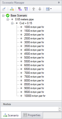
Figure 6: The Scenario Manager on the Quick Access Panel can be used to set up multiple throughput cases for a given solids concentration
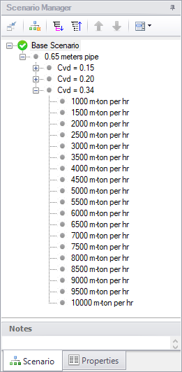
Figure 7: The Scenario Manager on the Quick Access Panel can be used to clone scenarios to easily create additional constant solids concentration cases
Setup the scenarios for constant throughput as follows:
-
Under the 0.65 meters pipe scenario, create a scenario called Flow = 3500 m-ton per hr. Load this scenario, and set the flow value in the Assigned Flow junction 3500 m-ton/hr.
-
Under the Flow = 3500 m-ton per hr scenario, create scenarios for a range of solids concentrations, as shown in Figure 8. Load each of these scenarios and set the solids concentration value in the Slurry Definition panel in Analysis Setup to the corresponding solids concentration value for each scenario.
-
Right-click scenario Flow = 3500 m-ton per hr and select Clone With Children. Name the new scenario Flow = 4000 m-ton per hr. In this scenario, set the flow value in the Assigned Flow junction 4000 m-ton/hr. Repeat this process, and create a set of scenarios for Flow = 4500 m-ton per hr.
-
There are now three additional sets of scenarios, each for a different throughput value. Each of the three flows will have a set of scenarios for a range of different solids concentrations, as shown in Figure 9.
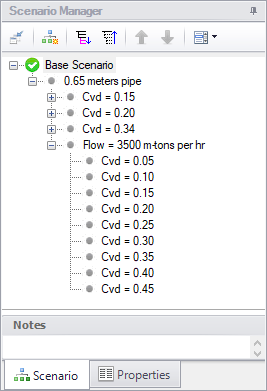
Figure 8: The Scenario Manager on the Quick Access Panel can be used to set up multiple solid concentration cases for a given throughput
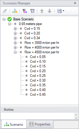
Figure 9: The Scenario Manager on the Quick Access Panel can be used to clone scenarios to easily create additional constant throughput cases
Step 9. Specify Output
Make sure that the Base Scenario is active, the open Output Control by selecting Output Control from the toolbar or Tools menu.
Knowing that for this example, the output data will be exported to a spreadsheet application, use the output control to set up the slurry output in a way that will make it simpler to plot the data in the spreadsheet. Open Output Control and on the Display Parameters tab, click the Slurry button. Then select the specific data to be displayed on the Slurry tab in the Output Window, as well as the order in which the data appears.
Figure 10 illustrates how the slurry output data could be organized in the Output Window. Because we will be plotting Jm vs. velocity in the spreadsheet, velocity and Jm are displayed next to each other in the output. One might also wish to plot Im vs. velocity, so velocity can be displayed again adjacent to the output data for Im.
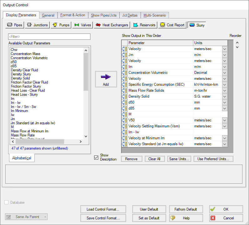
Figure 10: The Output Control window can be used to configure the slurry output into a format convenient for importing into a spreadsheet application
For this example, the multi-scenario output feature can also be used to simplify exporting the output data to a spreadsheet application. This feature allows the output from multiple scenarios to be viewed simultaneously. Load the 1000 m-ton per hr scenario that is under the Cvd = 0.15 scenario. Open the Output Control window and select the Multi-Scenario tab. Under Display Type, click Selected Scenarios and the Select Scenarios window appears. Check the box beside each scenario for which data is to be displayed in the Output, as shown in Figure 11. 84 of 92 scenarios should be selected. Click OK when finished.
Under Scenario Name Format, select Show Scenario Ancestral Name. Under Display Current Scenario, select In the Order Listed, if not selected already. Click the Clear All Colors button to make all scenario rows white.
This information should now appear, as shown in Figure 12. Close the Output Control window by clicking OK.
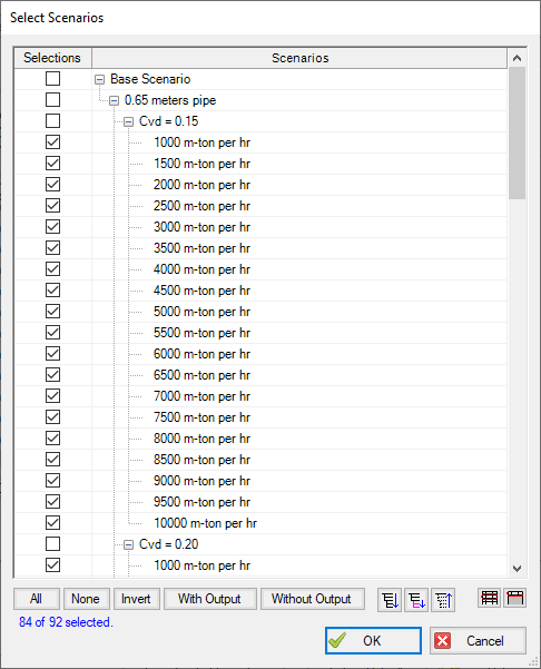
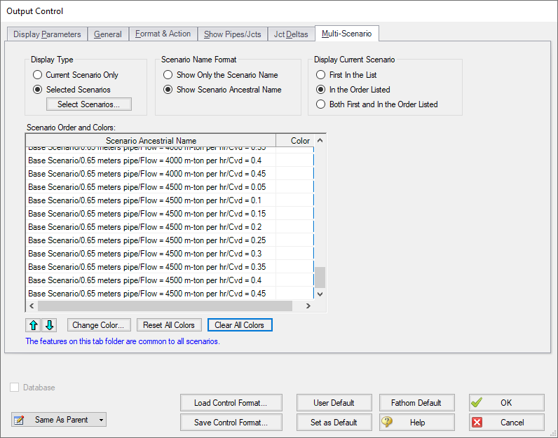
Figure 12: The Output Control window can be used to display the output from multiple scenarios simultaneously
Step 10. Run the Model
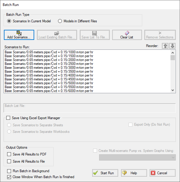
All of the different cases that have been set up for this example in each of the scenarios must now be run so the results can be examined. Because there are so many scenarios, the Batch Run feature in the File menu can be used to make running all of the different scenarios much easier.
From the File menu, select Start Batch Run. Under Batch Run Type, Scenarios In Current Model should be selected. Click Add Scenarios, and in the Select Scenarios window, select all 84 of the scenarios to be run, then click OK. All of the selected scenarios will be displayed in the Scenarios to Run list, as shown in Figure 13.
Click Start Run to start the analysis. The batch run manager will load and run each of the listed scenarios sequentially.
Step 11. Examine the Output
Once the batch manager has finished running all of the selected scenarios, load the scenario in which the multi-scenario output was set up (1000 m-ton per hr scenario that is under the Cvd = 0.15 scenario).
The Output window contains all the data that was specified in the Output Control window. Because the multi-scenario output feature was selected, it will also display the calculated output for each of the selected scenarios simultaneously. Figure 14 shows the multi-scenario output on the Slurry tab.
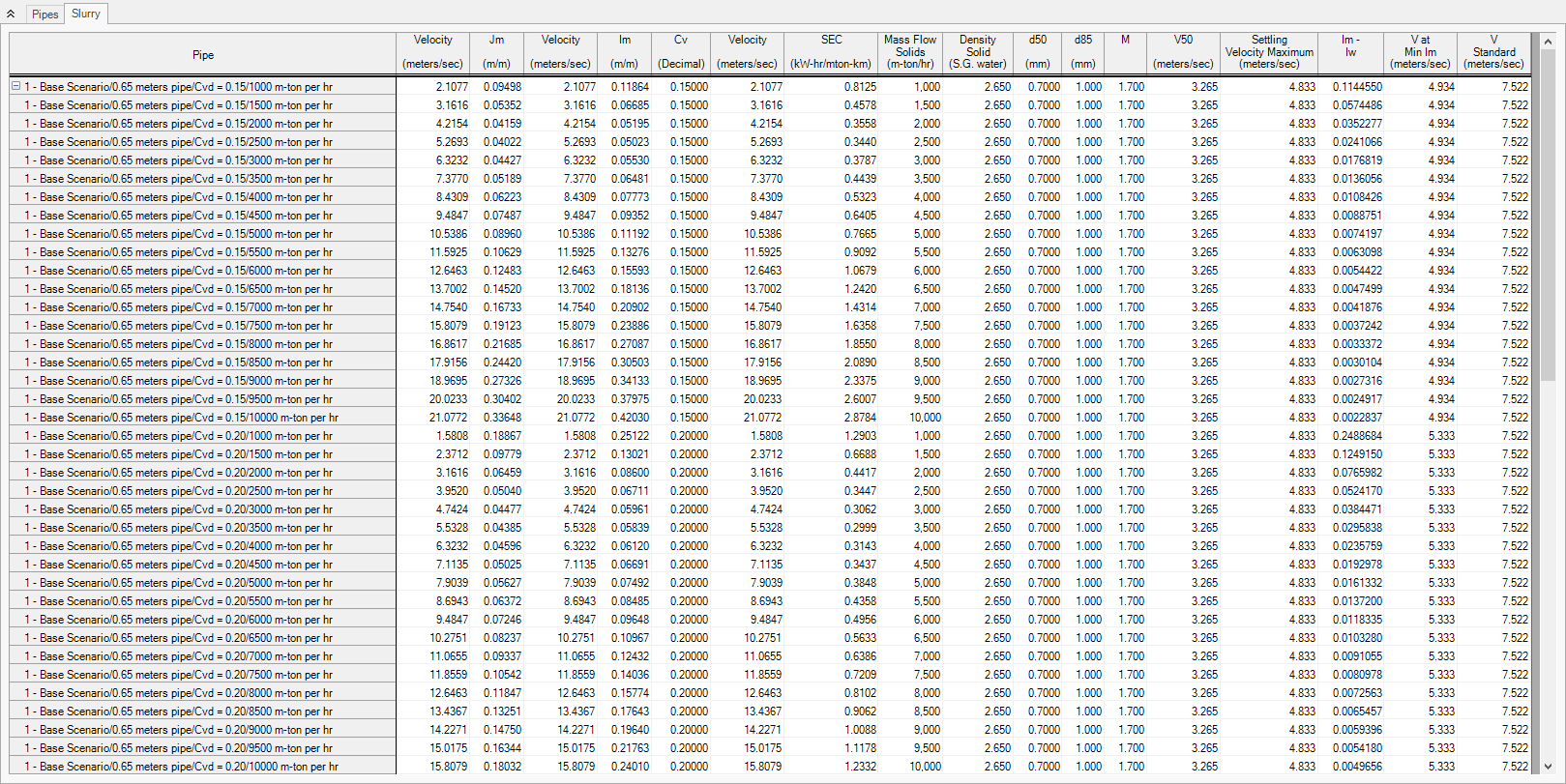
Figure 14: The Output window shows the Slurry results table in the center Pipes section for multiple scenarios
Step 12. Transfer the Output Data to a Spreadsheet
The information displayed on the Slurry tab in the Output window can be copied and pasted directly into a spreadsheet application, such as Excel, as shown in Figure 15. If the scenarios and the output were set up carefully, the data will already be formatted in such a way that graphing the information using the spreadsheet graphing features can be extremely straightforward.
Using the data in the spreadsheet, plot the Jm vs. velocity data for the three lines of constant solids concentration, and the three lines of constant solids throughput, as shown in Figure 16.
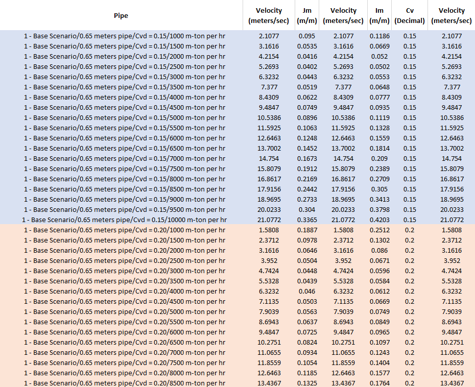
Figure 15: The Slurry results table in the Output window can be copied and pasted into a spreadsheet application in order to utilize the graphing features of the spreadsheet to generate the slurry system curves
Step 13. Analyze the Results
The results are shown in Figure 16. The solid lines refer to the constant solids concentration cases, and the broken lines refer to the constant throughput cases.
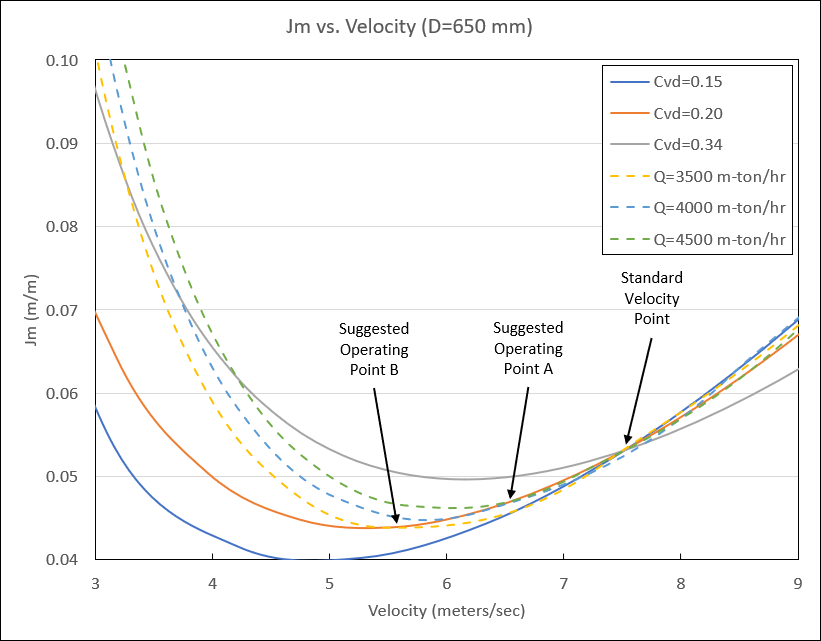
The arrows on the graph indicate the proposed operating conditions for the system on the 4000 m-ton/hr constant throughput line.
It is evident from the system characteristics that the proposed operating point Condition B, with the lower specific energy consumption, does not represent a feasible operating point for this slurry system. The system characteristics show the Jm decreasing as the mean velocity increases, so the operation would be unstable.
Even the first proposed operating condition, Condition A, is marginal. If the pump has a variable speed drive, and the solids concentration of the system does not fluctuate very much, this operating point could be used. However, as Figure 16 shows, if the concentrations vary from 3500 m-ton/hr to 4500 m-ton/hr, then the system operation is close to unstable for Condition A as well.
In order to allow for fluctuations in solids concentrations during system operations, and still maintain stable operation, it would be better to operate closer to the standard velocity. The standard velocity point is also shown in Figure 14 at about 7.5 m/s.
For this case, if operability is also considered, lower slurry concentrations, and higher energy consumption should be used to ensure system stability. Further, as discussed in the original reference, a different diameter pipe can be considered. The original reference suggests 0.55 m pipe as a better option than 0.65 m pipe because of operation closer to the standard velocity and lower capital cost.