PD Pulsation Study - PFA (English Units)
PD Pulsation Study - PFA (Metric Units)
Summary
A system with positive displacement pumps has a known pulsation issue in a section of piping with a closed valve. This issue is caused by the system’s natural frequency matching up with certain PD pump frequencies, resulting in severe pressure oscillations at the closed valve. Use AFT Impulse and the PFA (Pulsation Frequency Analysis) module to discover the problematic pump frequencies and what the pressure response at the closed valve is at these specific pump frequencies.
Note: This example can only be run if you have a license of the PFA module
Topics Covered
-
Ringing systems to find natural acoustic frequencies
-
Finding system excitation frequencies
-
Determining 'worst case' PD pump speeds at excitation frequencies
-
Calculating pressure response of system at above PD speeds
Required Knowledge
This example assumes the user has already worked through the Walk-Through Examples section, and has a level of knowledge consistent with the topics covered there. If this is not the case, please review the Walk-Through Examples, beginning with the Beginner: Valve Closure example. You can also watch the AFT Impulse Quick Start Video (English Units) on the AFT website, as it covers the majority of the topics discussed in the Valve Closure example.
This example is based on the paper by James M. Blanding and Trey Walters.
Model File
This example uses the following file, which is installed in the Examples folder as part of the AFT Impulse installation:
Step 1. Start AFT Impulse
From the Start Menu choose the AFT Impulse 9 folder and select AFT Impulse 9.
To ensure that your results are the same as those presented in this documentation, this example should be run using all default AFT Impulse settings, unless you are specifically instructed to do otherwise.
Step 2. Define the Modules Panel
First the PFA add-on modules needs to be activated for use in the model. To do this, open Analysis Setup from the toolbar or Analysis menu. On the Modules panel, check the box next to Activate PFA. After the PFA module is activated, the Use option should being selected by default.
Step 3. Define the Fluid Properties Group
Open the Fluid panel then define the fluid:
-
Fluid Library = User Specified Fluid
-
Name = PFA Fluid
-
Density = 57.3 lbm/ft3
-
Dynamic Viscosity = 2.3 lbm/hr-ft
-
Bulk Modulus = 140,000 psia
Step 4. Define the Pipes and Junctions Group
At this point, the first two groups are completed in Analysis Setup. The next undefined group is the Pipes and Junctions group. To define this group, the model needs to be assembled with all pipes and junctions fully defined. Click OK to save and exit Analysis Setup then assemble the model as shown in the figure below.
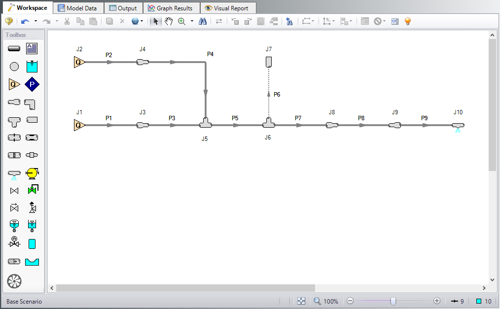
The system is in place but now we need to enter the input data for the pipes and junctions. Double-click each pipe and junction and enter the following data in the properties window.
Pipe Properties
-
Pipe Material = (User Specified)
-
Inner Diameter = Use table below
-
Length = Use table below
-
Wavespeed = User Specified Wavespeed
-
Wavespeed = 3000 feet/sec
-
-
Friction Model Data Set = User Specified
-
Selection = Absolute Roughness
-
Value = 0.0006 inches
| Pipe | Inner Diameter (inches) | Length (feet) |
|---|---|---|
| 1 | 12 | 3 |
| 2 | 12 | 3 |
| 3 | 2.157 | 39 |
| 4 | 2.157 | 57 |
| 5 | 3.26 | 33 |
| 6 | 1.682 | 21 |
| 7 | 3.26 | 48 |
| 8 | 1.682 | 3 |
| 9 | 3.26 | 30 |
Junction Properties
Note: For the sake of simplicity, assigned flow junctions J1 and J2 are being used to represent the PD pumps. The Pulsation Setup window will be used later to place the necessary transient data in the assigned flow junction for the pump being analyzed.
-
Assigned Flows J1 & J2
-
Elevation = 0 feet
-
Volumetric Flow Rate = 35.5 gal/min
-
-
Area Changes J3 & J4
-
Inlet Elevation = 0 feet
-
Type = Abrupt Transition (Cylindrical)
-
-
Tee/Wye J5 & J6
-
Elevation = 0 feet
-
Loss Model = Simple (no loss)
-
-
Dead End J7
-
Elevation = 0 feet
-
-
Area Changes J8 & J9
-
Inlet Elevation = 0 feet
-
Type = Conical Transition
-
Angle (μ) = 90 degrees
-
-
Spray Nozzle J10
-
Elevation = 0 feet
-
Loss Model = Cd Spray (Discharge Coefficient)
-
Geometry = Spray Nozzle
-
Exit Properties = Pressure
-
Exit Pressure = 0 psig
-
Cd (Discharge Coefficient) = 1
-
Discharge Flow Area = 0.02313 inches2
-
ØTurn on the Show Object Status from the View menu to verify if all data is entered. If so, the Pipes and Junctions group in Analysis Setup will have a check mark. If not, the uncompleted pipes or junctions will have their number shown in red. If this happens, go back to the uncompleted pipes or junctions and enter the missing data.
Step 5. Define the Pulsation Setup Group
Defining the initial pulse or ring is an important step in determining the natural frequencies that different stations in the model will respond to. This is the numerical equivalent of hitting the system with a hammer to see how it responds at different frequencies. This first step does not represent a realistic operating condition, but rather reveals what frequencies of real world operation may present operational problems.
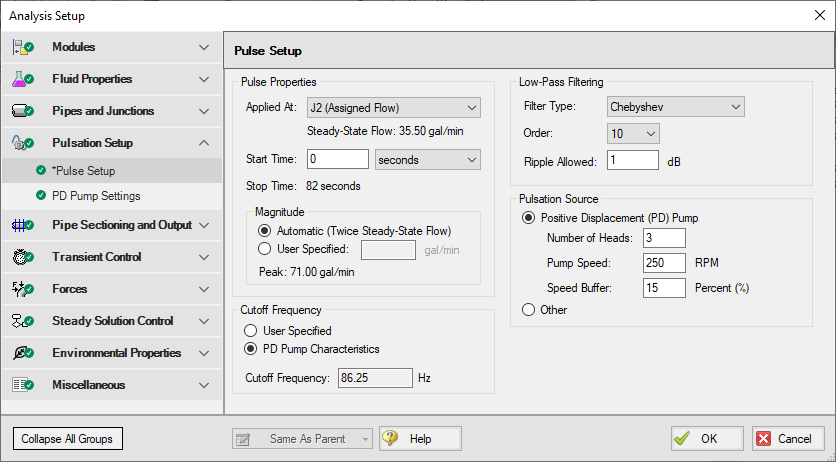
Open Analysis Setup to see the Pulsation Setup group below the Transient Control group. Use the Pulsation Setup group to specify input regarding the initial pulse and other information about the pulsation source. There are two panels in the Pulsation Setup group: the Pulse Setup and PD Pump Settings panels. The PD Pump Settings panel only requires input if the source of pulsation is a positive displacement pump. Because the source of pulsation in our model is a positive displacement pump, we will need to complete the input on both of these tabs. Enter the data below to define the Pulse Setup panel.
-
Applied At = J2 (Assigned Flow)
-
Start Time = 0 seconds
-
Magnitude = Automatic (Twice Steady-State Flow)
-
Peak = 71.00 gal/min
-
Cutoff Frequency = PD Pump Characteristics
-
Filter Type = Chebyshev
-
Order = 10
-
Ripples Allowed = 1 dB
-
Pulsation Source = Positive Displacement (PD) Pump
-
Number of Heads = 3
-
Pump Speed = 250 RPM
-
Speed Buffer = 15 Percent (%)
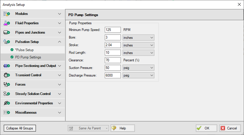
Now that all required input has been entered in the Pulse Setup panel, enter the following information on the PD Pump Settings panel (see Figure 3).
-
Minimum Pump Speed = 125 RPM
-
Bore Diameter = 3 inches
-
Stroke = 2.04 inches
-
Rod Length = 10 inches
-
Clearance = 70 Percent (%)
-
Suction Pressure = 50 psig
-
Discharge Pressure = 6000 psig
Step 6. Define the Pipe Sectioning and Output Group
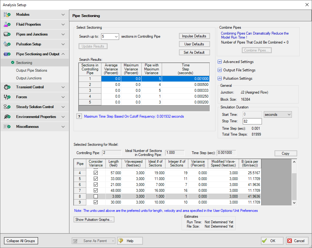
Open the Sectioning panel in Analysis Setup. While using the AFT Impulse PFA module, the pulsation setup needs to be completed prior to sectioning the pipes in the model. To section the model’s pipes for the simulation, complete the following:
-
Select the significant pipes that should consider wavespeed variance. In this example we will consider the variance in all modeled pipes, except for Pipe P8. You can see that this pipe has been excluded in Figure 4. Pipe P8 is excluded because it represents a flow meter and not an actual pipe. Units such as flow meters and dampeners may be better modeled with a pipe than with a junction if they have significant length and associated acoustic interaction aspects in the physical system. Ensure that the box next to each pipe is selected under Consider Variances, except for Pipe P8.
-
Click Update Results and select one section in the controlling pipe by clicking on one section in the table under Search Results. This window is displayed in Figure 4.
-
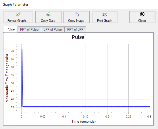
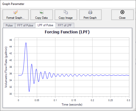
Select Show Pulsation Graphs located at the bottom left of the Sectioning panel. A graph of the pulse will appear (see Figure 5). You can also view graphs for the FFT of the Pulse, the LPF of the Pulse FFT, and the FFT of the LPF in the Graph Parameter graph that appears. The LPF of Pulse is shown in Figure 6. After you are done viewing these graphs, click Close to return to the Section Pipes window.
-
Click OK to save and close Analysis Setup.
-
Click OK for the pop-up window notifying you that the forcing function has been placed on J2 (the junction that was selected in the Pulsation Setup window) as transient data.
-
Open J2 to verify that the numerical ring has been applied to the transient (see Figure 7 for the transient input). This transient is a brief jump in flow rate at junction J2.
![]()
Figure 7: Assigned Flow Properties with Transient from Pulsation Setup. The Show Graph button under the Transient Data table can be selected to view the graph of this data
Step 7. Run the Model
Click Run Model from the toolbar or from the Analysis menu. This will open the Solution Progress window. This window allows you to watch the progress of the Steady-State and Transient Solvers. When complete, click the Graph Results button at the bottom of the Solution Progress window.
Step 8. Examine the Results
-
Find excitation frequencies to study
-
On the Graph Control tab in the Quick Access Panel, click the Frequency tab to begin generating an Excitation Frequency Analysis graph
-
We need to determine which frequencies excite the pump speeds within the pump speed range we have specified. For the purposes of this example, we will graph the Excitation Frequency graph for 10 different pipe stations. Note that it is the engineer's responsibility to evaluate all pipe stations that could be excited by various frequencies and to perform the necessary analysis.
-
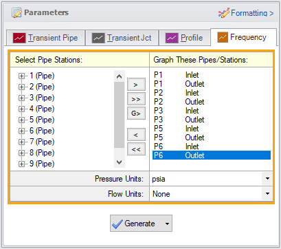
On the Graph Results tab, select the Frequency tab and select the inlet and outlet stations for the following pipes: 1, 2, 3, 5, and 6 (see Figure 8).
-
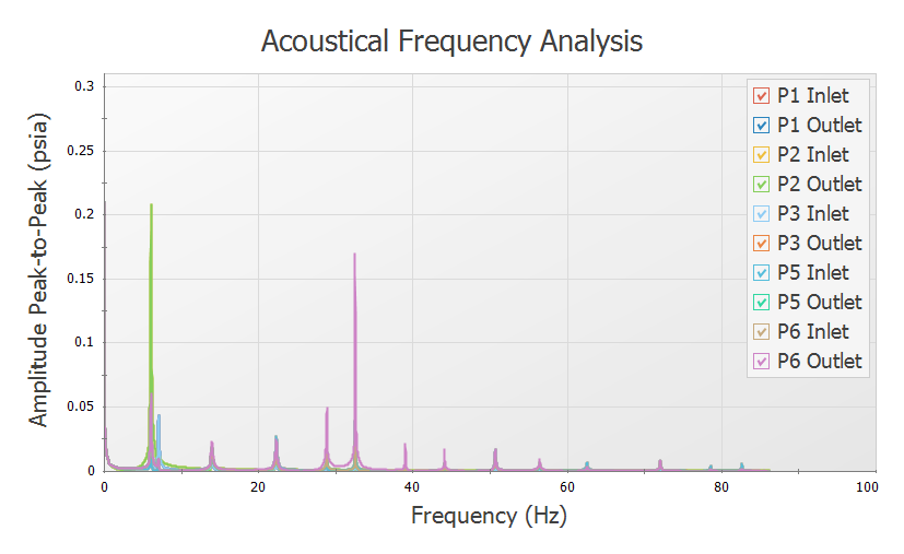
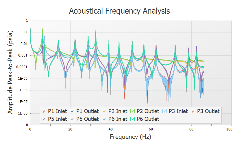
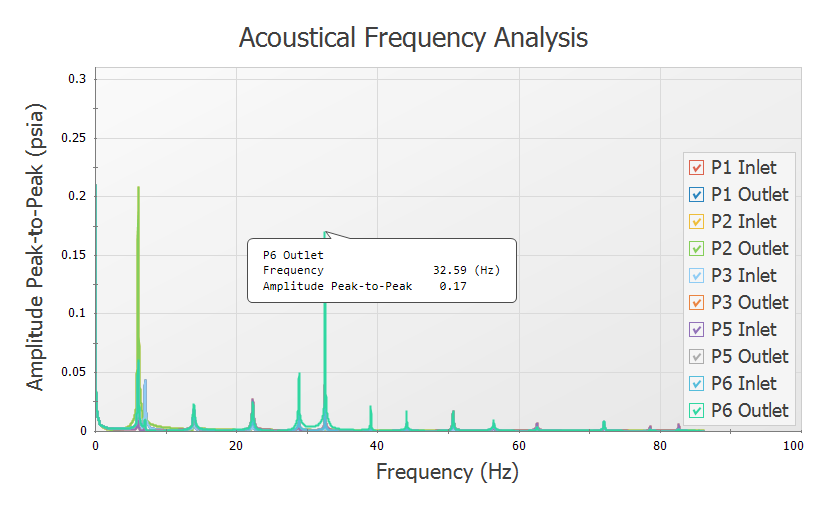
Click Generate. The resulting graph (shown in Figure 9) represents the frequencies that are excited by the pulse defined in the Pulsation Setup window.
-
From the graph in Figure 9, we see that there are several frequencies that produce a large pressure magnitude. Points on the plot with a large response magnitude are easily identified by finding local maxima on the graph. These maxima are the acoustic natural frequencies that are potentially the most damaging when excited by the identified pump speeds.
-
Note that the graph in Figure 9 can quickly be changed to display the magnitude on a logarithmic scale in order to allow for easier viewing of the magnitude behavior changes with a changing frequency. To view the Excitation Frequency Analysis graph with the magnitude displayed on a logarithmic scale, generate the frequency graph as discussed above. Right-click on either axis and select the box next to Logarithmic. See Figure 10 for an image of the graph in Figure 9 with the amplitude changed to be displayed on a logarithmic scale.
-
Evaluate excitation frequencies
-
The identified frequencies can now be evaluated to determine pump speeds that would cause them to be excited, making them potentially problematic. Follow the steps below to select and evaluate the excitation frequencies.
-
Left-click near the frequency of about
-
-
Right-click on the dialog flag that appears on the peak of this frequency as shown in Figure 12.
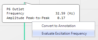
-
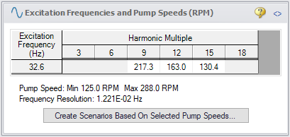
Select Evaluate Excitation Frequency to add this frequency to the Pump RPM Evaluation panel, which is labeled with Excitation Frequencies and Pump Speeds (RPM) (see Figure 13)
-
Repeat steps a through c for the local maxima at the frequencies of
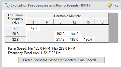
Figure 14: Pump RPM Evaluation Panel with Excitation Frequencies and their Harmonic Multiples Displayed
-
When choosing low or high frequencies on the graph, it is possible to select a frequency which is excited in the system but does not have a pump speed within the minimum and maximum pump speeds for the analysis. The minimum pump speed is defined directly in the PD Pump Settings in the Pulsation Setup window, while the maximum is calculated using the Pump Speed and Speed Buffer defined under Pulsation Source in Pulsation Setup. For example, try selecting the largest maxima, which occurs at 6.1 Hz. The message in Figure 15 appears.
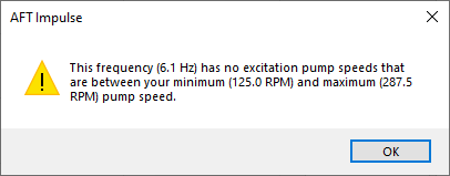
Figure 15: Message Indicating No Excitation Pump Speeds Between the Minimum and Maximum Pump Speeds Exist
-
Determine the pressure response of the system at excited frequencies
-
In the Pump RPM Evaluation panel, corresponding pump speeds can be selected for study. At these speeds, the pressure response is important to characterize. By default, all speeds in the Pump RPM Evaluation panel are pre-selected and must be clicked to be turned off. Scenarios can then be created that will use the information from the PD Pump Settings to create a child Pump Speed scenario that will have the Flow vs. Time profile at the selected speed (RPM) that will excite the evaluated frequencies.
-
We will create child scenarios for all six pump speeds in the Pump RPM Evaluation panel. To do this, ensure that all pump speeds are selected (not italicized).
-
Click Create Scenarios Based On Selected Pump Speeds…
-
A dialog box will appear stating that six scenarios will be created based on the selected speeds in the Pump RPM Evaluation panel. Click Yes to continue creating the child scenarios.
-
Load the
-
The scenario will now have different transient information in J2, modeling the pump performance at
-
Run the
-
To create a pressure profile graph in pipe P6, go to the Graph Results tab and select Profile for the graph type
-
Check the box for Pipe P6
-
Select Pressure Stagnation for the Parameter
-
Use
-
Click Generate
Figure 17 shows the profile plot for Pipe P6 at a pump speed of
The pressure vs. time can be displayed for any pipe station. Plot the pressure vs. time for pipe P6 by following the directions below:
-
In the Quick Access Panel, select Transient Pipe for the graph type
-
Expand the pipe station menu for Pipe P6
-
Add the outlet and inlet of Pipe P6 to the Graph These Pipes/Stations list
-
Select Pressure Stagnation for the Parameter
-
Use
-
Set the Time Frame to User Specified with a Start Time of 0 and a Stop Time of 2 seconds.
-
Click Generate (see Figure 18).
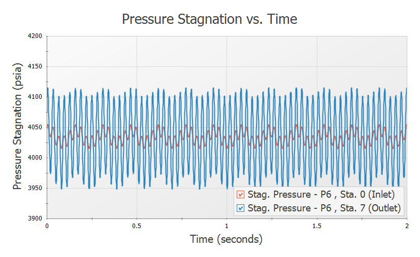
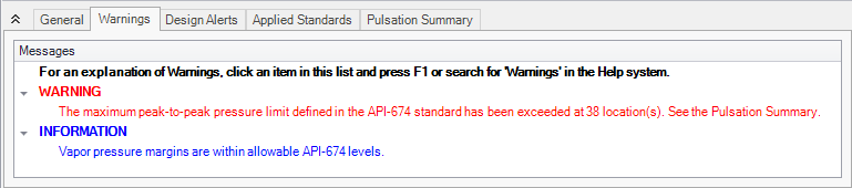
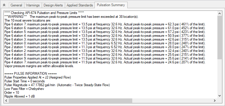
After looking at these graphs, go to the Output tab, which should open to the Warnings tab. The PFA module will check the Peak-to-Peak pressures and compare them to the permissible values in the API-674 standard. If the limits from the standard are violated in the model, a warning will appear. In this case, the the Peak-to-Peak pressures exceed the allowable limits. See Figure 19. Additionally, the vapor pressure margin is checked. This is the margin between the minimum pressure and 10% over the vapor pressure, per the API-674 standard. For a full summary, click on the Pulsation Summary tab, as is shown in Figure 20.
For the purposes of this example, we will repeat these steps for the pump speed of
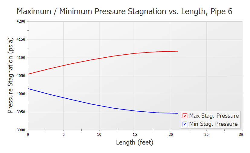
Figure 21 shows the Max/Min Pressure Profile for P6 for the pump speed of
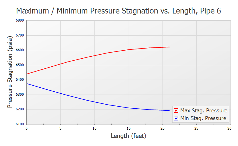
Notice the large difference between the maximum and minimum pressures at the end of the pipe, located next to the Dead End junction.
Figure 22 shows the Max/Min Pressure Profile for P6 for the pump speed of
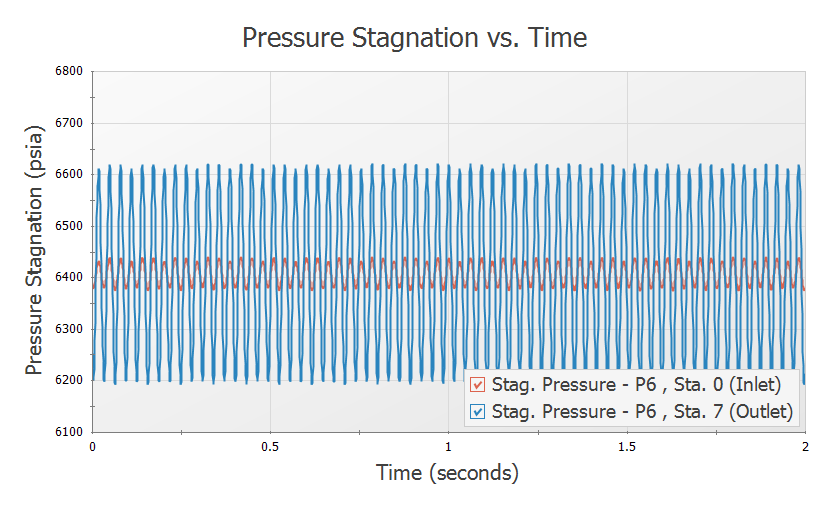
The large pressure oscillation in Pipe P6 can be seen in Figure 22. It is important to note that the inlet of Pipe P6 does not exhibit as large of a response as the outlet does. This oscillation, if allowed to continue, can lead to mechanical and support fatigue and thus failure.
Return to the Output tab of the Graph results window for the scenario with the pump speed of
PFA Analysis Summary
AFT Impulse and the PFA (Pulsation Frequency Analysis) module were used to discover the problematic pump frequencies occurring in a system with a known pulsation issue. The software was used to identify these frequencies, and after the frequencies were identified, a corresponding pump operating speed was examined to find the pressure response of the system. Using graphing features, the pressure response was plotted and studied. The steps followed lead to the successful pulsation analysis of the system.


