Positive Displacement Pump (Metric Units)

Summary

This example is designed to illustrate how to model the rapid cycling flow for a positive displacement pump with AFT Impulse. Models of a duplex and triplex positive displacement pump will be analyzed.

Topics Covered

• Using Repeat Transient feature on a pump

• Modeling submerged pumps

• Using the Gas Accumulator junction

Required Knowledge

This example assumes the user has already worked through the Beginner: Valve Closure example, or has a level of knowledge consistent with that topic. You can also watch the AFT Impulse Quick Start Video (English Units) on the AFT website, as it covers the majority of the topics discussed in the Valve Closure example.

Model File

This example uses the following file, which is installed in the Examples folder as part of the AFT Impulse installation:

• US - Positive Displacement Pump.imp

Step 1. Start AFT Impulse

From the Start Menu choose the AFT Impulse 9 folder and select AFT Impulse 9.

To ensure that your results are the same as those presented in this documentation, this example should be run using all default AFT Impulse settings, unless you are specifically instructed to do otherwise.

Step 2. Define the Fluid Properties Group

1. Open Analysis Setup from the toolbar or from the Analysis menu.

2. Open the Fluid panel then define the fluid:

   1. Fluid Library = AFT Standard

   2. Fluid = Water (liquid)

      1. After selecting, click Add to Model

   3. Temperature = 60 deg. F

Step 3. Define the Pipes and Junctions Group

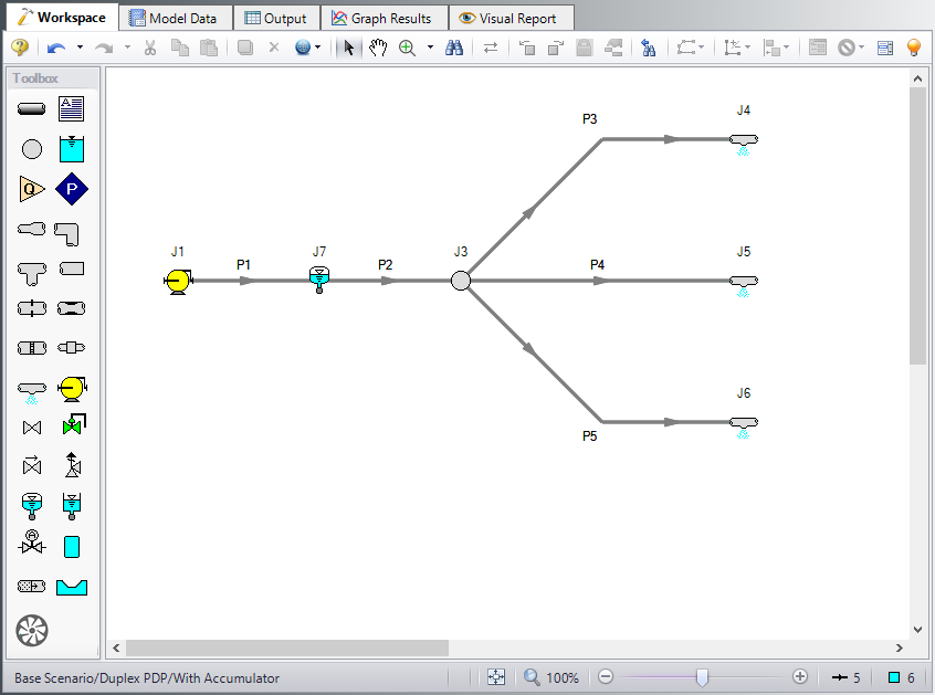
At this point, the first two groups are completed in Analysis Setup. The next undefined group is the Pipes and Junctions group. To define this group, the model needs to be assembled with all pipes and junctions fully defined. Click OK to save and exit Analysis Setup then assemble the model as shown in the figure below.

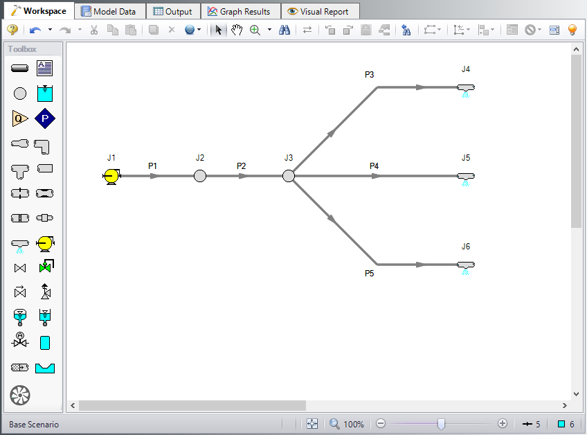
The system is in place but now we need to enter the input data for the pipes and junctions. Double-click each pipe and junction and enter the following data in the properties window.

Pipe Properties

1. Pipes P1 & P2

   1. Pipe Material = Steel - ANSI

   2. Size = 1-1/2 inch

   3. Type = XS (schedule 80)

   4. Friction Model Data Set = Standard

   5. Length = 5 feet

   6. Wavespeed = Calculated Wavespeed

2. Pipes P3 - P5

   1. Pipe Material = (User Specified)

   2. Inner Diameter = 1.5 inches

   3. Wall Thickness = 0.15 inches

   4. Modulus of Elasticity = 3,000,000 psia

   5. Poisson Ratio = 0.3

   6. Length = 100 feet

   7. Wavespeed = Calculated Wavespeed

   8. Friction Model Data Set = User Specified

   9. Selection = Absolute Roughness

   10. Value = 0.002 inches

Junction Properties

1. Pump J1

   1. Inlet Elevation = 0 feet

   2. Pump Model = Positive Displacement

   3. Parameter = Volumetric Flow Rate

   4. Flow Rate = Steady

   5. Steady Flow rate = 100 gal/min

   6. Submerged Pump = Checked

   7. Selection = Head (HGL)

   8. Liquid Surface HGL = 3 feet

2. Branches J2 & J3

   1. Elevation = 0 feet

3. Spray Discharges J4 - J6

   1. Elevation = 0 feet

   2. Loss Model = Cd Spray (Discharge Coefficient)

   3. Geometry = Spray Nozzle

   4. Exit Properties = Pressure

   5. Exit Pressure = 0 psig

   6. Cd (Discharge Coefficient) = 0.6

   7. Discharge Flow Area = 0.05 inches2

ØTurn on the Show Object Status from the View menu to verify if all data is entered. If so, the Pipes and Junctions group in Analysis Setup will have a check mark. If not, the uncompleted pipes or junctions will have their number shown in red. If this happens, go back to the uncompleted pipes or junctions and enter the missing data.

Step 4. Define the Pipe Sectioning and Output Group

ØOpen Analysis Setup and open the Sectioning panel. When the panel is first opened it will automatically search for the best option for one to five sections in the controlling pipe. The results will be displayed in the table at the top. Select the row to use one section in the controlling pipe. 

Step 5. Define the Transient Control Group

ØOpen the Simulation Mode/Duration panel in the Transient Control group. Enter 5 seconds for the Stop Time.

All groups should now be complete and the model is ready to run. If all groups in Analysis Setup have a green checkmark then Click OK and proceed. Otherwise, enter the missing information.

Step 6. Create Child Scenarios

In this model we want to evaluate four displacement pump cases: Duplex and Triplex, each without and with an accumulator.

A. Create the Duplex Scenarios

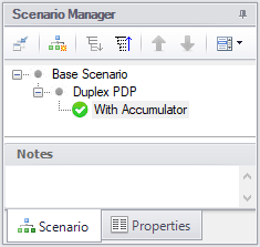
Using the Scenario Manager on the Quick Access Panel, create a child scenario by either right-clicking on the Base Scenario and then selecting Create Child, or by first selecting the Base Scenario on the Scenario Manager on the Quick Access Panel and then selecting the Create Child icon. Enter the name Duplex PDP. A new scenario will appear below the Base Scenario in the list. Select the Duplex scenario and create another child and call it With Accumulator. See Figure 2.

B. Set up the Duplex PDP Scenario

In the Scenario Manager load the Duplex PDP scenario.

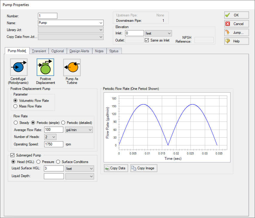
ØOpen the J1 Pump junction and do the following:

1. Flow Rate = Periodic (simple)

2. Average Flow Rate = 100 gal/min

3. Number of Heads = 2

4. Operating Speed = 1490 rpm

The periodic flow rate for the duration of one period will be shown. Impulse will continuously repeat this flow rate cycle throughout the transient, using the average flow rate as the initial steady-state flow rate.

The window should appear as in Figure 3. Click OK to exit the window. This scenario is now completed.

C. Commentary on modeling positive displacement pumps

For this example the pump flow vs. time data has been based on an idealized case, where the time varying flow may be represented as half sine waves for each pump cylinder (half is discharge while the other half of the cycle is suction), one sine wave for each cylinder phased according to the number of cylinders (e.g. 180 degrees for a duplex pump, 120 degrees for a triplex pump). This can be viewed by opening the pump junctions, to see the graph on the Pump Model tab. One will note that the flow for the duplex pump varies from a maximum value to zero flow since each cylinder discharges over 180 degrees of rotation and the two cylinders are 180 degrees out of phase. By comparison, the flow from the individual cylinders of the triplex pump, 120 degrees out of phase, overlap so that minimum flow is greater than zero. Real positive displacement pumps deviate from a sine wave due to the effects of valving and leakage. Accordingly, it is preferable to use manufacturer data when available.

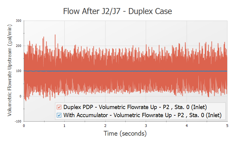
Initial, steady-state flow rate is typically specified based on the nominal flow rate of the pump. Often, one may see a difference between this flow rate and the flow rate as displayed in Graph Results. This difference will typically derive from two sources; 1) differences between a manufacturer's time vs. flow curves and the nominal pump rating and, 2) differences resulting from stepwise integration of the time varying flow. In the case of calculating time varying flow based on an idealized sine wave, the latter will occur because the calculated data points are based on a different stepwise integration basis than performed by AFT Impulse during the analysis. A similar result occurs based on the number of data points taken from a published curve. An example of this difference can be seen in the Duplex PDP with Accumulator scenario by graphing flow in the pipe after the accumulator (P2). Initial flow begins at the specified steady-state value of 100 gal/min, but decreases over time to a steady-state value slightly less than this (~1 gal/min). It takes a few seconds in this example for the flow to stabilize since the initial accumulator pressure has been calculated based on the initial flow specified for the pump. As the integrated time varying flow is slightly different, system resistance is different than the initial conditions and the accumulator must come to a different pressure to balance this resistance. A change in accumulator pressure is coupled with a net outflow or inflow of liquid in the accumulator, which takes time.

Finally, this example deals only with modeling discharge piping, but what about suction piping? In this example we didn't need to model suction piping to the pump since we selected the optional, 'Submerged Pump' modeling. We could have modeled suction piping supplying the pump and it would be subjected to the same time varying flow variation as the discharge. Modeling the system this way will result in the suction and discharge flows being in phase, whereas in the actual system suction and discharge flows are out of phase. In most situations this difference is not significant since the suction and discharge sides of the system are hydraulically isolated from each other by the pump itself. In other words, one can consider the suction and discharge sides of the piping system as two, distinct systems. In those cases where it is desired to model the out of phase relationship of the suction and discharge flows, the pump can be split in two, so to speak, a suction and discharge half. This example already includes the discharge half so that the suction half could be modeled as an assigned flow junction along with the suction piping. Time varying flow can be specified for an assigned flow junction in the same way as the pump in this example. One would modify the time vs. flow data to reflect the out of phase nature of the suction flow.

D. Set up the With Accumulator Scenario

Now we want to add an accumulator junction to review the effects on pressure and transients. In the Scenario Manager load the With Accumulator scenario

1. Morph the J2 Branch into a Gas Accumulator.

   1. Hold down the CTRL key on the keyboard.

   2. While continuing to hold down the key, drag a gas accumulator junction from the Toolbox and drop it on the J2 Branch.

   3. Let go of the CTRL key. The gas accumulator junction should take on the number J7. See Figure 4.

2. Double-click the J7 Gas Accumulator to open the properties window.

3. Polytropic Constant in Transient = 1.2

4. Initial Gas Volume = Known Volume

5. Value = 0.2 feet3

This scenario is now completed.

E. Set up the Triplex PDP scenario

From this point we can create the Triplex scenario by cloning the Duplex PDP scenario.

1. In the Scenario Manager select the Duplex PDP scenario

2. Right click the scenario name and select the Clone With Children menu item

3. Name the scenario Triplex PDP. This scenario will have a child called With Accumulator. Leave this scenario as is

4. Double-click the Triplex PDP scenario to load it as the current scenario

5. Open the Pump J1 properties window

6. Change the Number of Heads to 3

7. The periodic flow rate for the duration of one period will be shown. Impulse will continuously repeat this flow rate cycle throughout the transient, using the average flow rate as the initial steady state flow rate.

8. Click OK.

This scenario is now completed.

Step 7. Run the Model

Using the Scenario Manager, load each scenario and run it. This can also be accomplished by performing a batch run from the File menu.

Note that once the scenarios are run, a warning will be shown in each of the duplex pump scenarios stating that the Positive Displacement Pump added negative pressure. This is occurring due to the fact that the simple transient used in the positive displacement pump allows the flow in the pump to drop to zero throughout the transient, which requires a negative head rise across the positive displacement pump. Using a more realistic transient would likely resolve this warning.

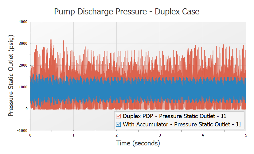
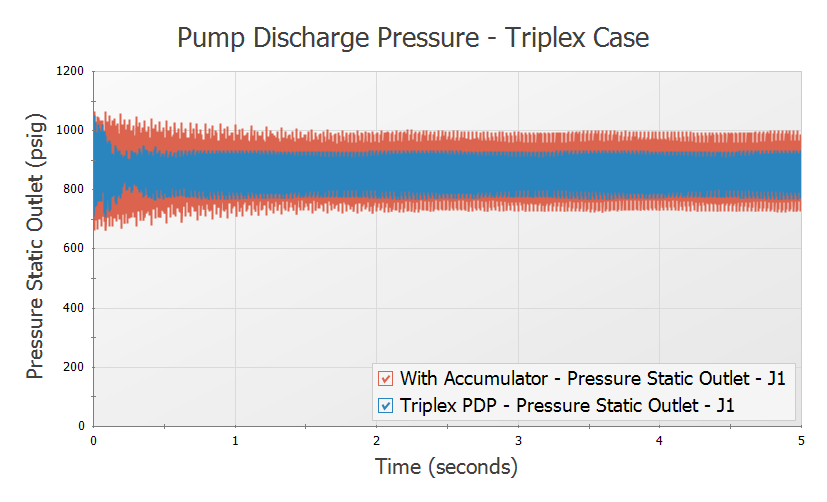
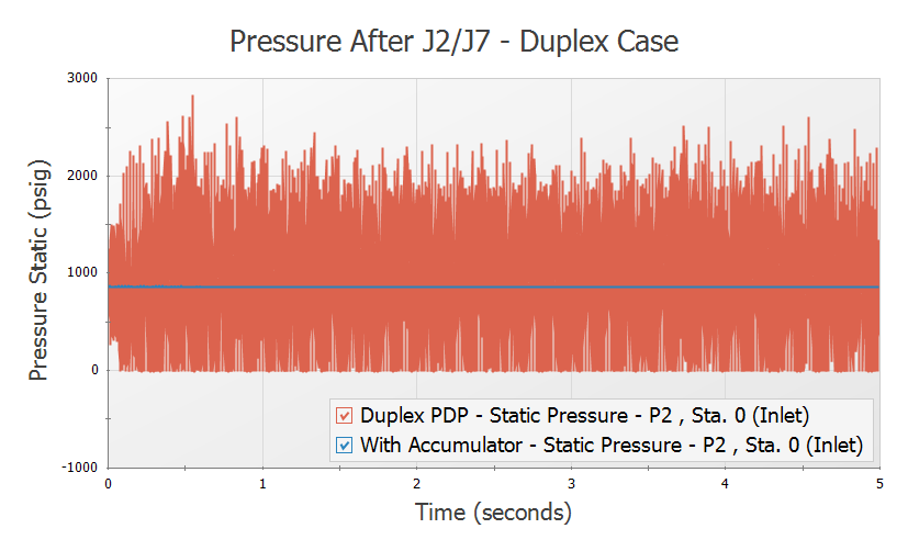
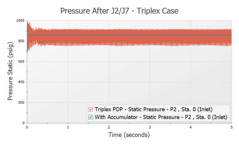
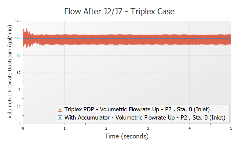
Step 8. Graph the Results

Graphs of the pressure and flow transients can be created for each scenario. The pump discharge pressures are shown in Figure 5 and Figure 6. The pressures at the J2 Branch & J7 Accumulator are shown in Figure 7 and Figure 8. The flows after the J2 Branch & J7 Accumulator are shown in Figure 9 and Figure 10.