Pump with Variable Speed Flow Control (Metric Units)

Summary

A pump with a variable speed drive for flow control supplies water to two heat exchangers. The flow to one of the exchangers is turned off, and the controlled pump flow rate is reduced by half over five seconds.

Topics Covered

• Using a variable speed controller on a pump

• Modeling a controlled flow rate transient for a pump

Required Knowledge

This example assumes the user has already worked through the Beginner: Valve Closure example, or has a level of knowledge consistent with that topic. You can also watch the AFT Impulse Quick Start Video (English Units) on the AFT website, as it covers the majority of the topics discussed in the Valve Closure example.

Model File

This example uses the following file, which is installed in the Examples folder as part of the AFT Impulse installation:

• US - Pump with Variable Speed Flow Control.imp

Step 1. Start AFT Impulse

From the Start Menu choose the AFT Impulse 9 folder and select AFT Impulse 9.

To ensure that your results are the same as those presented in this documentation, this example should be run using all default AFT Impulse settings, unless you are specifically instructed to do otherwise.

Step 2. Define the Fluid Properties Group

1. Open Analysis Setup from the toolbar or from the Analysis menu.

2. Open the Fluid panel then define the fluid:

   1. Fluid Library = AFT Standard

   2. Fluid = Water (liquid)

      1. After selecting, click Add to Model

   3. Temperature = 100 deg. F

Step 3. Define the Pipes and Junctions Group

At this point, the first two groups are completed in Analysis Setup. The next undefined group is the Pipes and Junctions group. To define this group, the model needs to be assembled with all pipes and junctions fully defined. Click OK to save and exit Analysis Setup then assemble the model as shown in the figure below.

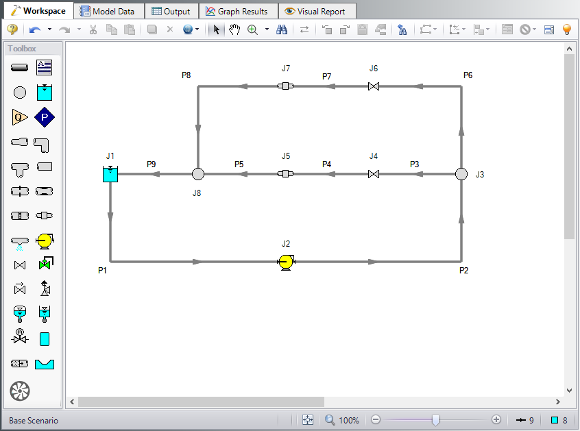
The system is in place but now we need to enter the input data for the pipes and junctions. Double-click each pipe and junction and enter the following data in the properties window.

Pipe Properties

1. Pipe Model tab

   1. Name = Use table below

   2. Pipe Material = Steel - ANSI

   3. Size = Use table below

   4. Type = STD (schedule 40)

   5. Friction Model Data Set = Standard

   6. Length = Use table below

Pipe	Name	Size	Length (feet)
1	Pump Suction Pipe	10 inch	30
2	Pump Discharge Pipe	10 inch	500
3	Pipe	8 inch	5
4	Pipe	8 inch	5
5	Pipe	8 inch	10
6	Pipe	8 inch	5
7	Pipe	8 inch	5
8	Pipe	8 inch	10
9	Pipe	10 inch	500

Junction Properties

1. Reservoir J1

   1. Name = Cooling Pond

   2. Tank Model = Infinite Reservoir

   3. Liquid Surface Elevation = 20 feet

   4. Liquid Surface Pressure = 0 psig

   5. Pipe Depth = 20 feet

2. Pump J2

   1. Name = Main Pump

   2. Inlet Elevation = 0 feet

   3. Pump Model tab

      1. Pump Model = Centrifugal (Rotodynamic)

      2. Performance Curve Used in Simulation = Standard Pump Curve

      3. Enter Curve Data

Volumetric	Head
gal/min	feet
0	60
2000	55
4000	40
5000	30

4. Curve Fit Order = 2

4. Variable Speed tab

   1. Pump Speed = Controlled Pump (Variable Speed)

   2. Selection = Volumetric Flow Rate

   3. Control Setpoint = 2000 gal/min

5. Transient tab

   1. Transient = Setpoint vs. Time

   2. Transient Special Condition = None

   3. Initiation of Transient = Time

   4. Transient Data = Absolute Values

Time (seconds)	Vol. Flow (gal/min)
0	2000
5	1000
10	1000

3. Branches J3 & J8

   1. Elevation = 0 feet

4. Valve J4

   1. Name = Valve #1

   2. Inlet Elevation = 0 feet

   3. Cv = 500

5. General Components J5 & J7

   1. J5 Name = HEX #1

   2. J7 Name = HEX #2

   3. Inlet Elevation = 0 feet

   4. Loss Model = Resistance Curve

   5. Enter Curve Data =

Volumetric	Head
gal/min	feet
0	0
1000	20
2000	80

6. Curve Fit Order = 2

6. Valve J6

   1. Name = Valve #2

   2. Inlet Elevation = 0 feet

   3. Loss Model tab

      1. Cv = 500

   4. Transient tab

      1. Transient Special Conditions = None

      2. Initiation of Transient = Time

      3. Transient Data = Absolute Values

Time (seconds)	Cv
0	500
0.5	100
1	0
10	0

ØTurn on the Show Object Status from the View menu to verify if all data is entered. If so, the Pipes and Junctions group in Analysis Setup will have a check mark. If not, the uncompleted pipes or junctions will have their number shown in red. If this happens, go back to the uncompleted pipes or junctions and enter the missing data.

Step 4. Define the Pipe Sectioning and Output Group

ØOpen Analysis Setup and open the Sectioning panel. When the panel is first opened it will automatically search for the best option for one to five sections in the controlling pipe. The results will be displayed in the table at the top. Select the row to use one section in the controlling pipe. 

Step 5. Define the Transient Control Group

ØOpen the Simulation Mode/Duration panel in the Transient Control group. Enter 10 seconds for the Stop Time.

Step 6. Run the Model

Click Run Model from the toolbar or from the Analysis menu. This will open the Solution Progress window. This window allows you to watch the progress of the Steady-State and Transient Solvers. When complete, click the Graph Results button at the bottom of the Solution Progress window.

Step 7. Graph the Results

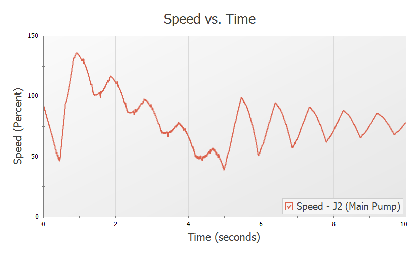
Figure 2 shows the speed history for the J2 Main Pump while it adjusts from 2,000 gal/min to 1,000 gal/min.

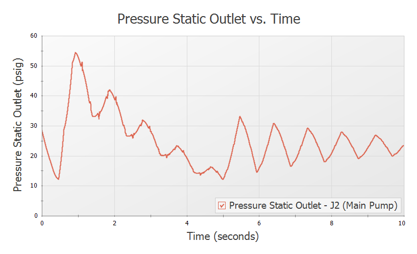
Figure 3 shows the pressure history for the J2 Main Pump discharge.

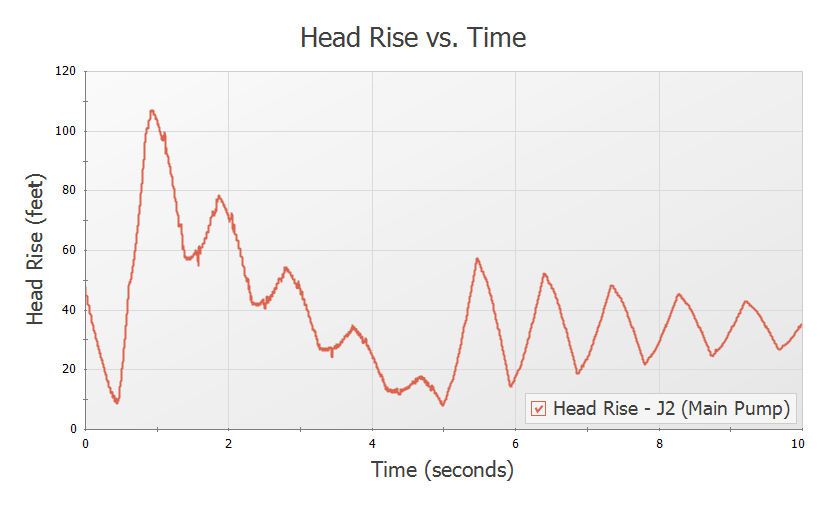
Figure 4 shows the head rise across the pump.

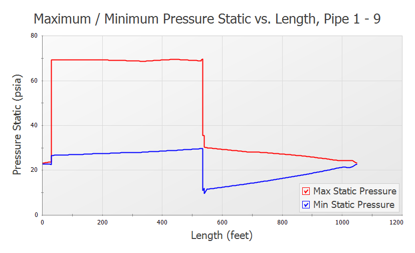
Choosing a flow path through the J7 Hex #2, a pressure profile is shown in Figure 5.