Tank Farm with Infinite Pipes (Metric Units)

Summary

A long supply pipeline flows into a gasoline tank farm. The transient occurs when flow is switched from one storage tank to another. Two scenarios compare the results with and without an infinite pipe boundary, and also compares the run times.

Topics Covered

• Using infinite pipes

Required Knowledge

This example assumes the user has already worked through the Beginner: Valve Closure example, or has a level of knowledge consistent with that topic. You can also watch the AFT Impulse Quick Start Video (English Units) on the AFT website, as it covers the majority of the topics discussed in the Valve Closure example.

Model File

This example uses the following file, which is installed in the Examples folder as part of the AFT Impulse installation:

• US - Tank Farm with Infinite Pipes.imp

Step 1. Start AFT Impulse

From the Start Menu choose the AFT Impulse 9 folder and select AFT Impulse 9.

To ensure that your results are the same as those presented in this documentation, this example should be run using all default AFT Impulse settings, unless you are specifically instructed to do otherwise.

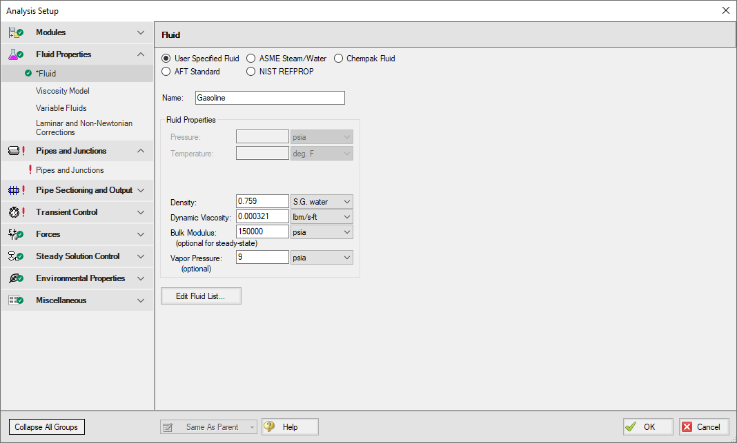
Step 2. Define the Fluid Properties Group

1. Open Analysis Setup from the toolbar or from the Analysis menu.

2. Open the Fluid panel then define the fluid:

   1. Fluid Library = User Specified Fluid

   2. Name = Gasoline

   3. Density = 0.759 S.G. water

   4. Dynamic Viscosity = 0.000321 lbm/s-ft

   5. Bulk Modulus = 150000 psia

   6. Vapor Pressure = 9 psia

Step 3. Define the Pipes and Junctions Group

At this point, the first two groups are completed in Analysis Setup. The next undefined group is the Pipes and Junctions group. To define this group, the model needs to be assembled with all pipes and junctions fully defined. Click OK to save and exit Analysis Setup then assemble the model as shown in the figure below.

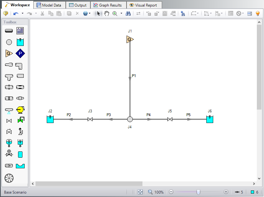
The system is in place but now we need to enter the input data for the pipes and junctions. Double-click each pipe and junction and enter the following data in the properties window.

Pipe size and lengths, as well as junction elevation data are given below. Here we see that the inlet assigned flow junction represents the flow coming from a pumping station that is 30 miles away. If the pumps in the pump station interact with the tank farm transients, then the pumps must be modeled in detail. We will find out later that they do not, and thus we can simplify the model by using an assigned flow junction at the pump discharge. The WEB Valve is initially closed. The way we represent this in steady-state is using a Special Condition to close it. As for the transient, the initial data point for Cv must be zero.

Junction Properties

1. Assigned Flow J1

   1. Name = Pump Station Discharge

   2. Elevation = 966 feet

   3. Type = Inflow

   4. Flow Specification = Volumetric Flow Rate

   5. Flow Rate = 13500 barrels/hr

2. Reservoir J2

   1. Name = Desert Petroleum

   2. Liquid Surface Elevation = 1029 feet

   3. Liquid Surface Pressure = 0 psig

   4. Pipe Depth = 40 feet

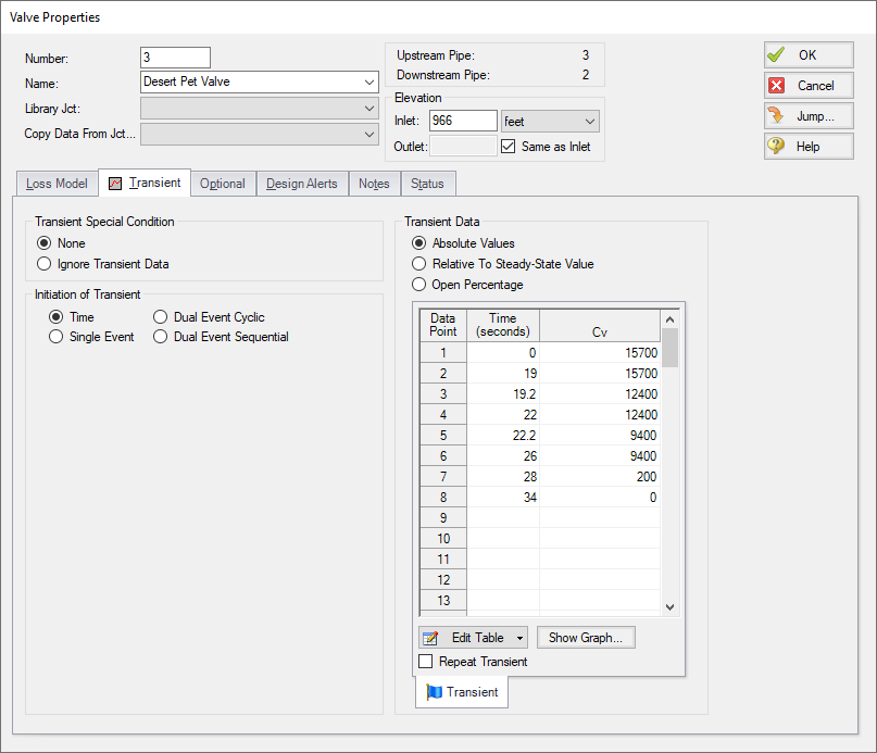
3. Valve J3

   1. Name = Desert Pet Valve

   2. Elevation = 966 feet

   3. Loss Model tab

      1. Valve Data Source = User Specified

      2. Loss Model = Cv

      3. Cv = 15700

   4. Transient tab

      1. Transient Special Condition = None

      2. Initiation of Transient = Time

      3. Transient Data = Absolute Values

Time (seconds)	Cv
0	15700
19	15700
19.2	12400
22	12400
22.2	9400
26	9400
28	200
34	0

4. Branch J4

   1. Elevation = 966 feet

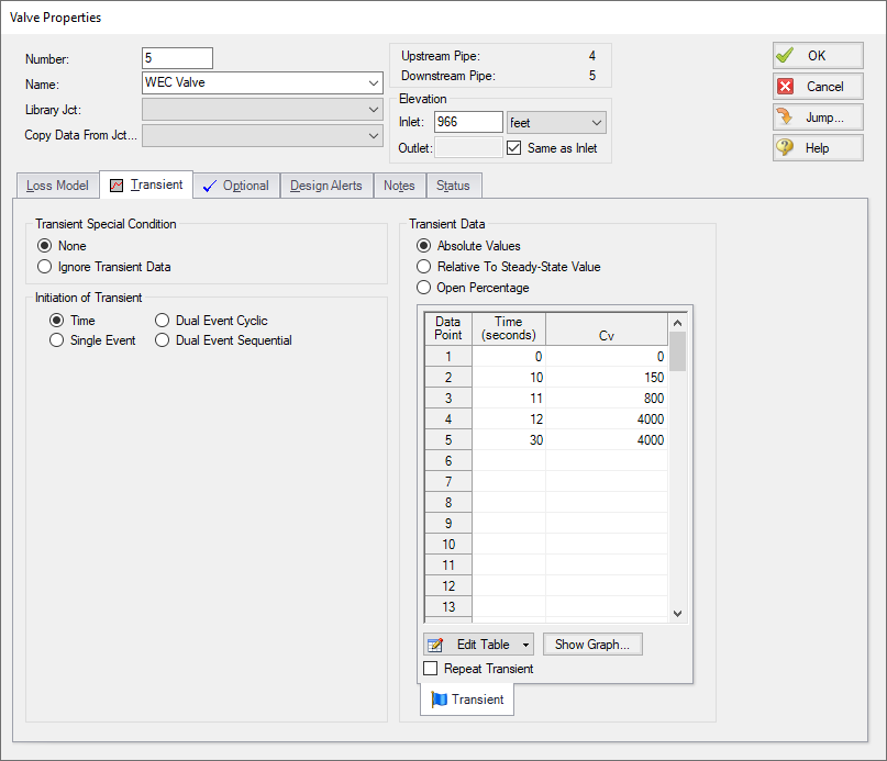
5. Valve J5

   1. Name = WEC Valve

   2. Elevation = 966 feet

   3. Loss Model tab

      1. Valve Data Source = User Specified

      2. Loss Model = Cv

      3. Cv = 4000

   4. Transient tab

      1. Transient Special Condition = None

      2. Initiation of Transient = Time

      3. Transient Data = Absolute Values

Time (seconds)	Cv
0	0
10	150
11	800
12	4000
30	4000

5. Optional tab

   1. Special Condition = Closed

6. Reservoir J6

   1. Name = West Coast Energy

   2. Tank Model = Infinite Reservoir

   3. Liquid Surface Elevation = 1023 feet

   4. Liquid Surface Pressure = 0 psig

   5. Pipe Depth = 0 feet

Pipe Properties

1. Pipe Model tab

   1. Pipe Material = Steel - ANSI

   2. Size = Use table below

   3. Type = schedule 40

   4. Friction Model Data Set = Standard

   5. Length = Use table below

Pipe	Size (inches)	Length
1	20	30 miles
2	20	300 feet
3	12	200 feet
4	12	30 feet
5	20	1000 feet

ØTurn on the Show Object Status from the View menu to verify if all data is entered. If so, the Pipes and Junctions group in Analysis Setup will have a check mark. If not, the uncompleted pipes or junctions will have their number shown in red. If this happens, go back to the uncompleted pipes or junctions and enter the missing data.

Step 4. Define the Pipe Sectioning and Output Group

ØOpen Analysis Setup and open the Sectioning panel. When the panel is first opened it will automatically search for the best option for one to five sections in the controlling pipe. The results will be displayed in the table at the top. Select the row to use one section in the controlling pipe. 

Step 5. Define the Transient Control Group

ØOpen the Simulation Mode/Duration panel. Enter the Stop Time as 35 seconds.

Step 6. Create Child Scenarios

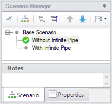
In this model we want to see the impact of using an infinite pipe boundary. We will do the comparison between two scenarios. In the Scenario Manager on the Quick Access Panel, create a child scenario by either right-clicking on the Base Scenario and then selecting Create Child, or by first selecting the Base Scenario on the Scenario Manager on the Quick Access Panel and then selecting the Create Child icon. Enter the name Without Infinite Pipe. A new scenario will appear below the Base Scenario in the list. Select the Base Scenario and create another child and call it With Infinite Pipe.

ØDouble-click the Without Infinite Pipe scenario in the list to load it as the current scenario, as shown by the green check mark icon, as shown in Figure 5.

Step 7. Run the First Scenario

This scenario models pipe P1 as 30 miles in length, which is its true length. Select Run Model from the toolbar or Analysis menu. The Waterhammer Assistant may open to inform you that using an Assigned Flow junction may not be appropriate. For our purposes it is appropriate, so click OK to dismiss the caution and to see the Solution Progress. This window allows you to watch the progress of Impulse Steady-State and Transient Solvers. Depending on the speed of your PC, this model may take several minutes to run. Note how long it takes so you can compare that to the other scenario later. Once finished, go to the Graph Results window.

Step 8. Graph the Results

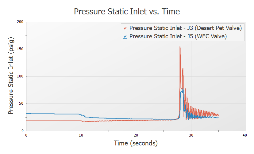
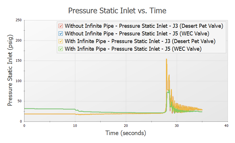
On the Graph Control tab of the Quick Access panel go to the Transient Jct tab. Add valves J3 and J5 to the junctions to be graphed (see Figure 6). Select as Pressure Static Inlet parameter and set the units to psig. Click Generate. This graphs the pressures at the valve inlets over time (see Figure 7). Save this graph to the Graph List by using the Add to Graph List button.

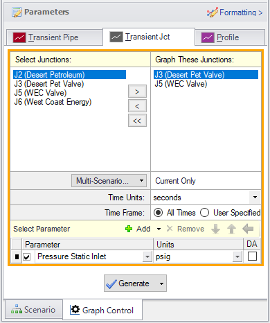
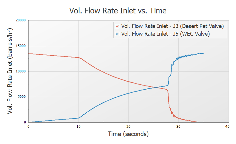
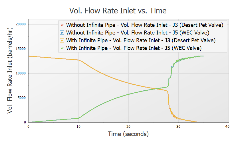
Now change the parameter to Vol. Flow Rate Inlet and set the units to barrels/hr. Click Generate. This graph shows the flowrates through the valves to each tank during the transient. Save this graph to the Graph List also.

Step 9. Consider an Infinite Pipe

The longest pipe in the system is the 30-mile pipe P1. If you open the Section Pipes window you will see it has over 5,000 computing sections, which is over 100 times as many as all the other computing sections combined. Thus the computation time for this model is dominated by pipe P1.

The wavespeed for pipe P1 is 3579 feet/sec, and the time frame for the simulation is 35 seconds. During the simulation any transients in the tank farm can propagate 125,265 feet (about 23.7 miles) up pipe P1 and thus never reach junction J1. For the J1 boundary to have any impact on the tank farm, it would have to receive the transient wave and then reflect its response back down pipe P1 to the tank farm. Thus the wave would have to travel 60 miles (i.e., up the pipe and then back), which would take 88.5 seconds.

The conclusion here is that any transients at the tank farm that take place in less than 88.5 seconds will not be affected by pipe P1 or junction J1. But one cannot neglect pipe P1, because flow is coming in from that pipe and transients are propagating up that pipe. This is an excellent opportunity to use an infinite pipe boundary. Infinite pipe boundaries accept all pressure waves but reflect none. If we use an infinite pipe boundary in this system, we will get virtually identical results for the first 88.5 seconds. If we let the model run longer than this, then the results will differ after that point in time. Since we are not interested in what happens after 88.5 seconds but only what happens up to 35 seconds, we can save a lot of computation time.

Step 10. Specify the Second Scenario

Load the With Infinite Pipe scenario and make the following changes:

1. Open the J1 Assigned Flow junction window.

2. Select the Transient tab.

3. In the Transient Special Conditions section, select No Reflections (Infinite Pipe).

4. Click OK.

5. Open the Pipe Properties window for pipe P1.

6. Change the length to 60 feet. The 60 feet length is somewhat arbitrary, and was chosen because the shortest pipe in the system (P4) is 30 feet long, and the pipe adjacent to the junction using the infinite pipe transient needs to have 2 sections. Thus modeling P1 as 60 feet does not affect the time step.

7. Click OK.

8. Open Analysis Setup and open the Sectioning panel.

9. Notice how pipe P1 now has two sections instead of over 5000.

10. Click OK.

Step 11. Run the Second Scenario

ØSelect Run Model from the toolbar or Analysis menu. This scenario runs much faster than the first one (about 1/60th as long).

Step 12. Graph the Results

Use the Graph List Manager to create the same graphs as before to compare results to the previous scenario. This can be done by loading the graphs from the Graph List Manager, then selecting both scenarios from the Multi-Scenario button in the Graph Parameters section and regenerating the graph. The results are practically identical for the two scenarios.

Conclusion

Using an infinite pipe boundary on the J1 Assigned Flow junction allowed us to obtain the same quality results at the tank farm with 1/60th of the computation time. While in this case the difference was between a few seconds versus a few minutes, a more complicated system could mean the difference between a one-hour run and a sixty-hour run.

Infinite pipe boundaries can also be employed on the Assigned Pressure junction type. The only difference is that during the steady-state the junction models a known pressure rather than a known flow. During the transient they function identically.

Finally, note that once the transient solution starts, the flow rate from an Assigned Flow junction and the pressure from an Assigned Pressure junction are no longer used. Both the flow rate and pressure at the junction will change over time, in a matter consistent with the fact that no reflections are occurring at that junction.