Valve Closure with Pipe Forces (Metric Units)

Summary

A gravity drain system transfers water from one tank to another through a filter and a valve in the connecting pipeline. It is necessary to determine the unbalanced transient forces that occur when the valve is partially closed in order to analyze pipe stresses and loads on the pipe supports.

Topics Covered

• Defining force sets

• Graphing transient forces

• Evaluating the effect of frictional losses on transient pipe forces

• Using the isometric pipe drawing mode

• Generating a CAESAR II force file

Required Knowledge

This example assumes the user has already worked through the Beginner: Valve Closure example, or has a level of knowledge consistent with that topic. You can also watch the AFT Impulse Quick Start Video (English Units) on the AFT website, as it covers the majority of the topics discussed in the Valve Closure example.

Model File

This example uses the following file, which is installed in the Examples folder as part of the AFT Impulse installation:

• US - Valve Closure with Pipe Forces.imp

Step 1. Start AFT Impulse

From the Start Menu choose the AFT Impulse 9 folder and select AFT Impulse 9.

To ensure that your results are the same as those presented in this documentation, this example should be run using all default AFT Impulse settings, unless you are specifically instructed to do otherwise.

Step 2. Define the Fluid Properties Group

1. Open Analysis Setup from the toolbar or from the Analysis menu.

2. Open the Fluid panel then define the fluid:

   1. Fluid Library = AFT Standard

   2. Fluid = Water (liquid)

      1. After selecting, click Add to Model

   3. Temperature = 70 deg. F

Step 3. Define the Pipes and Junctions Group

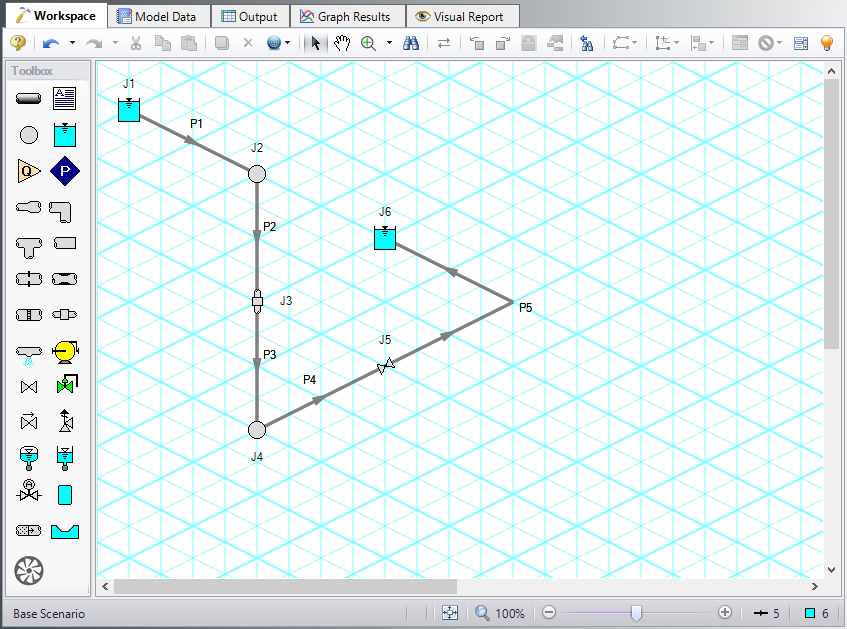
At this point, the first two groups are completed in Analysis Setup. The next undefined group is the Pipes and Junctions group. To define this group, the model needs to be assembled with all pipes and junctions fully defined. Click OK to save and exit Analysis Setup then assemble the model as shown in the figure below.

The previous examples’ models were drawn using the default Pipe Drawing Mode, 2D Freeform. However, AFT Impulse has two additional available drawing modes, 2D Orthogonal and Isometric. Due to the nature of this model it is more convenient to use the Isometric mode to visually interpret the pipe layout and have a better understanding of the system when interpreting calculated forces.

1. From the Arrange menu, select the option to Show Grid and choose Isometric under Pipe Drawing Mode.

2. Place the junctions as shown below in Figure 1.

3. Double-click the pipe tool and draw the pipes in the model as shown. When drawing segmented pipes such as P5, a red-dashed preview line will show how the pipe will be drawn on the isometric grid. As you are drawing a pipe, you can change the preview line by clicking any arrow key on your keyboard or scrolling the scroll wheel on your mouse.

Note: You can hold the ALT key while adjusting a pipe by the endpoint to add an additional segment. This can be used with the arrow key or mouse scroll wheel to change between different preview line options.

4. Align the junctions using the Rotate Icons buttons, or right click on the junctions and select Auto-rotate Icon to automatically align the junctions with the connected pipes. Alternatively, Customize Icon can be selected from the right click menu to manually choose an icon/orientation.

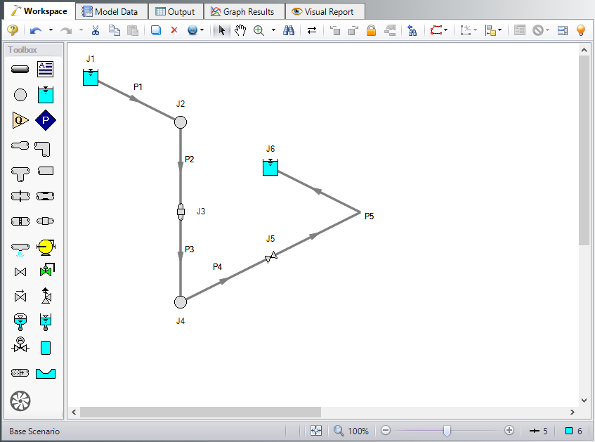
5. The grid can be shown or turned off in the Arrange menu, as shown in Figure 2.

The system is in place but now we need to enter the input data for the pipes and junctions. Double-click each pipe and junction and enter the following data in the properties window.

Pipe Properties

1. Pipe Model tab

   1. Pipe Material = Steel - ANSI

   2. Size = 20 inch

   3. Type = STD (schedule 20)

   4. Friction Model Data Set = Standard

   5. Length = Use table below

   6. Wavespeed = Calculated Wavespeed

Pipe	Length (feet)
1	480
2	20
3	20
4	480
5	80

Note: Pipe forces are typically calculated around pairs of pipe direction changes or at single points where the pipe is interrupted (for example, at an untied or non-pressure compensated expansion joint). These locations must be determined from piping drawings showing the physical arrangement of the piping and junction and then related to the corresponding pipe in the AFT Impulse model along with the length along the pipe where the direction change or pipe interruption is located. Intermediate elevations are not necessary but are included here for later discussion.

Junction Properties

1. Reservoir J1

   1. Tank Model = Infinite Reservoir

   2. Liquid Surface Elevation = 50 feet

   3. Liquid Surface Pressure = 0 psig

   4. Pipe Elevation = 40 feet

2. Branch J2

   1. Elevation = 40 feet

3. General Component J3

   1. Name = Filter

   2. Inlet Elevation = 20 feet

   3. Loss Model = K Factor

   4. K = 10

4. Branch J4

   1. Elevation = 0 feet

5. Valve J5

   1. Loss Model tab

      1. Inlet Elevation = 0 feet

      2. Valve Data Source = User Specified

      3. Loss Model = Cv

      4. Loss Source = Fixed Cv

      5. Cv = 13215

   2. Transient tab

      1. Transient Special Condition = None

      2. Initiation of Transient = Time

      3. Transient Data = Relative To Steady-State Values

Time (seconds)	% Cv of Steady State
0	100
2	10
10	10

6. Reservoir J6

   1. Liquid Surface Elevation = 10 feet

   2. Liquid Surface Pressure = 0 psig

   3. Pipe Elevation = 0 feet

ØTurn on the Show Object Status from the View menu to verify if all data is entered. If so, the Pipes and Junctions group in Analysis Setup will have a check mark. If not, the uncompleted pipes or junctions will have their number shown in red. If this happens, go back to the uncompleted pipes or junctions and enter the missing data.

Step 4. Define the Pipe Sectioning and Output Group

ØOpen Analysis Setup and open the Sectioning panel. When the panel is first opened it will automatically search for the best option for one to five sections in the controlling pipe. The results will be displayed in the table at the top. Select the row to use one section in the controlling pipe. 

Note: The closer computing stations are to the desired force calculation location the more accurate the force calculation will be.

Step 5. Define the Transient Control Group

ØOpen the Simulation Mode/Duration panel in the Transient Control group. Enter 10 seconds for the Stop Time.

Step 6. Define the Forces Group

ØOpen the Force Definitions panel and define a force set by clicking New, entering the name, the start pipe, length to start node, end pipe, and the length to end node. Repeat this process for the second force set as shown in Figure 3.

Note: Force sets can also be defined from the Workspace by right-clicking on the starting pipe(s) to automatically create a difference force set from the start node to the end node of that pipe. The force set can then be edited from the Transient Control window.

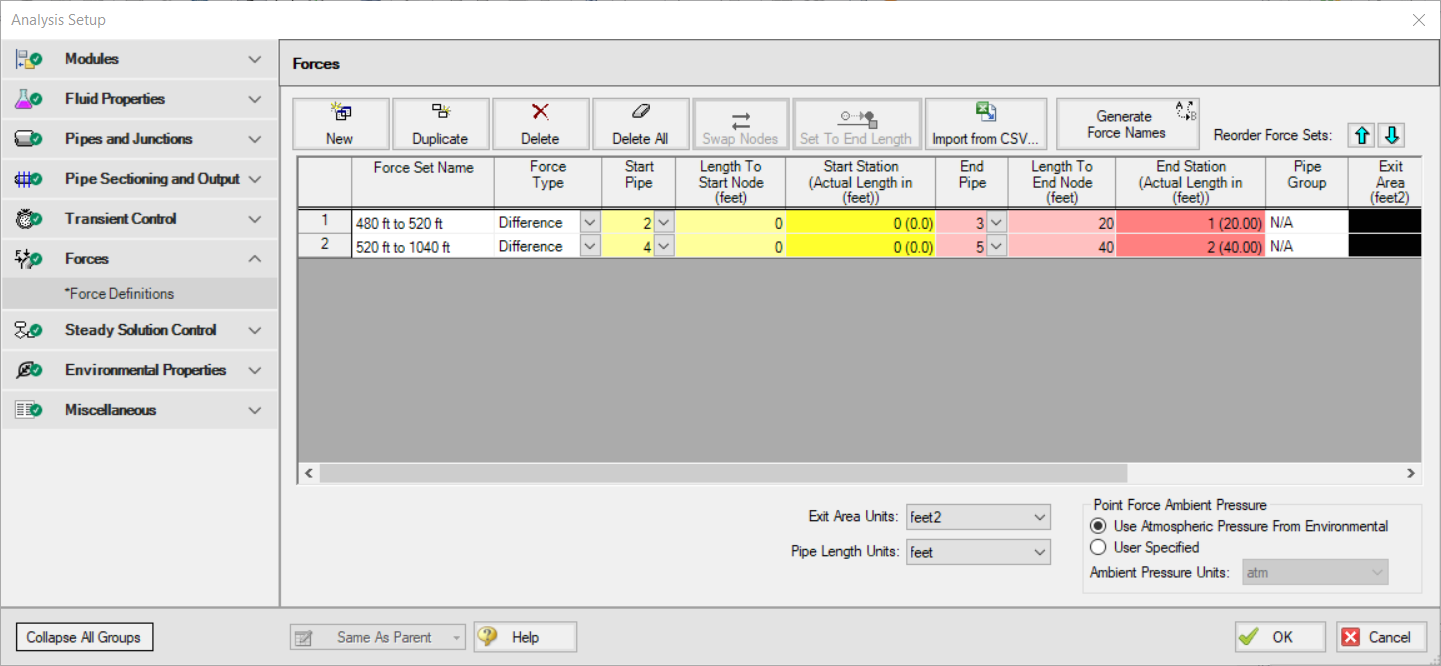
Since the force sets in this example calculate the force imbalance between adjacent pipe direction changes, the default force type of ‘Difference’ is used. The ‘Point’ type would be used for calculating the force at a location where the pipe is interrupted. The additional difference methods are available to analyze forces across more than two pipes, or for cases where a user defined exit area would be useful, such as for forces across a nozzle.

For a specified length to start node and length to end node, AFT Impulse will determine and display the nearest computing station number and actual length from inlet of the start and end pipe to the node within the pipe.

Sectioning has produced one section each in pipes P2 and P3 for the 480 feet to 520 feet force set and then 24 sections and four sections in pipes P4 and P5, respectively for the 520 feet to 1040 feet force set. Section length is 20 feet for each pipe.

In our example, this sectioning conveniently results in computing stations at the locations where we want to calculate forces. Where computing stations do not coincide with the desired force calculation locations, some loss in accuracy will occur. By increasing the number of sections in the controlling pipe during sectioning, a greater number of computing stations will exist, thus reducing the distance to the desired force calculation locations at the expense of longer run time.

Note: AFT Impulse will automatically set Pipe Station Output to include only those stations required by the force set nodes up to five. If more than five stations are required, all stations will be specified.

An Impulse model does not contain directional data with regard to the forces, it knows only pipe length and elevation. Since forces are vectors with both magnitude and direction, the user must identify the direction of the calculated forces using data in the pipe arrangement drawing that defines the geometry of the pipe routing. This directional information can then be entered using the Force Unit Vector columns. The force unit vectors will not impact Impulse's calculations, but may be useful if it is desired to export the Impulse force output to a pipe stress software as is discussed in step 8.

ØClick OK to save and close Analysis Setup.

Step 7. Run the Model

Click Run Model from the toolbar or from the Analysis menu. This will open the Solution Progress window. This window allows you to watch the progress of the Steady-State and Transient Solvers. When complete, click the Graph Results button at the bottom of the Solution Progress window.

Step 8. Graph the Results

ØOn the Quick Access Panel, in the Parameters section, select the Forces tab. The force sets defined on the Force Definitions panel will appear as available forces to graph.

Check the box next to the 480 ft to 520 ft force set. This corresponds to the elevation change between the branch junctions of 40 feet and 0 feet specified from pipes P2 and P3. Click Generate and the following force versus time graph is displayed (Figure 4).

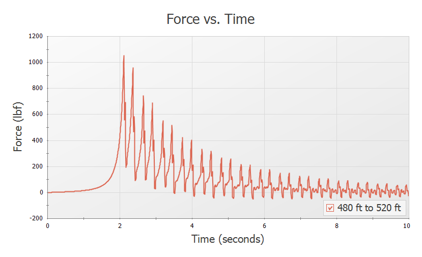
Note that at time 0, which represents the initial, steady state results, there is no force imbalance. This is the expected results for a system at steady state.

Some traditional methods of analyzing force sets will not have this same result, since they do not include the effects of friction or momentum in their force balances. If the graph from Figure 4 were created with friction and momentum ignored, the steady state value would be calculated as approximately -2700 lbf. Due to this effect, Impulse will always include both friction and momentum when calculating and graphing force sets.

Now create the same graph but for the 520 ft to 1040 ft force set. The resulting force vs time is shown in Figure 5.

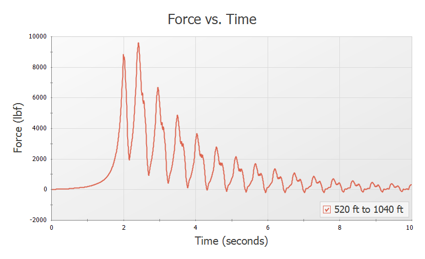
Again we see that with friction included there is no force imbalance under steady state conditions (time 0). If friction were not included in the force calculations as is done here a steady state imbalance of approximately -1270 lbf would have been observed.

There are two important points to be observed here:

1. AFT Impulse calculates transient, or time varying hydraulic forces. This does not include constant loads from fluid, piping, and fittings weight. A comprehensive analysis of pipe loading must separately include these items.

2. In some cases, ignoring friction and momentum force balance terms will result in force imbalances that do not exist in reality, since the frictional forces on the pipe exactly counterbalance the force calculated from the pressure differential at the selected locations.

Step 9. Export CAESAR II Force File

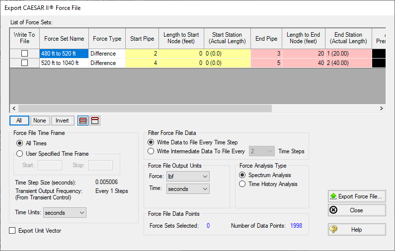
ØGo to the Output window, click on the File menu and select Export Force File and choose CAESAR II Force File , which will open the export file window shown in Figure 6.

The force sets to include in the force file may be individually selected, and all or only intermediate data points may be included in the force file. For the force sets and options selected the number of data points that will be in the file is displayed. This number should not exceed the maximum number of data points allowed in CAESAR II.

In addition if unit vector information has been entered for the force sets in the Transient Control window, the Export Unit Vector option can be used to include this information in the exported file.

Final Note

If transient cavitation occurs, the warning shown in Figure 7 will be displayed in the Output window:

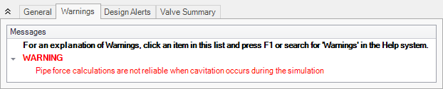
Calculating time varying forces requires a greater level of accuracy in the magnitude and location of pressures, velocity and frictional losses than may be determined with transient cavitation modeling. Accordingly, pipe force calculations will have a usually indeterminable reduction in accuracy when cavitation occurs.