Open vs. Closed Systems
Model a Closed Loop System
A closed circulating system can easily be modeled with AFT Impulse by locating a Reservoir junction anywhere in the system and setting the pressure to the known pressure at that point. Inflow and outflow pipes will then need to be connected. The Reservoir junction merely acts as a reference pressure against which all other pressures in the system are compared. Because there are no other inlets or outlets to the system, then whatever is delivered by the Reservoir junction to the system will also be received from the other pipes, thus achieving a net zero outflow rate for the system.
Balancing Mass
In order to model a closed system, only one pressure junction is used in the model. Typically this would be either a Reservoir or Assigned Pressure. Pressure type junctions are an infinite source of fluid and do not balance flow. How then can one be used to balance flow in a closed system?
To answer this question, it is worth considering how AFT Impulse views a closed system model. AFT Impulse does not directly model closed systems, and in fact does not even realize a closed system is being modeled.
Consider the system shown in Figure 1. This is an open system. Fluid is taken from J1 and delivered to J4 and J5. Because AFT Impulse’s Steady-State solution engine solves for a mass balance in the system, all flow out of J1 must be delivered to J4 and J5. Because the flow is steady-state, no fluid can be stored in the system; what goes in must go out.
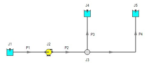
Figure 1: Open system - Flow out of J1 equals the sum of J4 and J5
Now consider the systems in Figure 2. The first system appears to be closed, while the second appears to be open. If the same boundary condition (i.e., surface elevation and pressure) is used for J1, J11 and J12 in the second system, to AFT Impulse it will appear as an identical system to the first system. The reason is that AFT Impulse takes the first system and applies the J1 reservoir pressure as a boundary condition to pipes P4, P9 and P10. The second system uses three reservoirs to apply boundary conditions to P4, P9 and P10. But if the reservoirs all have the same elevation and pressure, the boundary conditions are the same as J1 in the first system. Thus the same boundary condition is used for P4, P9 and P10 in both models, and they appear identical to AFT Impulse.
But how is the flow balanced at J1 in the first system? Looking at the first system, one sees that to obtain a system balance, whatever flows into P10 must come back through P4 and P9. Because there is overall system balance by the solver, it will give the appearance of a balanced flow at the pressure junction J1. If there is only one boundary (i.e., junction) where flow can enter or leave the pipe system, then no flow will enter or leave because there isn’t anywhere for it to go. Thus the net flow rate will be zero at J1 (i.e., it will be balanced). But recognize that AFT Impulse is not applying a mass balance to J1 directly. It is merely the result of an overall system balance.
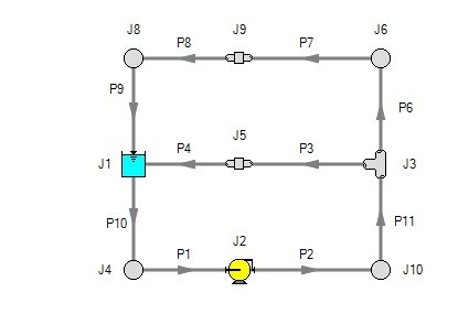
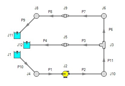
Figure 2: The first system is closed, and the second open. In both systems the flow into P10 is the same as sum of P4 and P9. If the second system has the same conditions at J1, J11 and J12, the two system will appear identical to AFT Impulse.


