Orifice Loss Model
Sharp-Edged Orifice
The orifice loss factors are all for turbulent Reynolds numbers. The sharp-edged orifice shown in Figure 1, is given by the following equation(Idelchik, 2007Idelchik, I. E., Handbook of Hydraulic Resistance, 4th edition, Begell House, Redding, CT, 2007., 259):

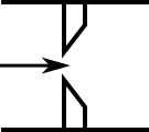
Figure 1: Sharp-edged orifice (in this case Aup = Adown)
Round-Edged Orifice with Different Upstream and Downstream Diameters
When the upstream and downstream pipe diameters are different for a round-edged orifice as shown in Figure 2, the round-edged orifice equation for different pipe areas is used and is given by the following (Idelchik, 2007Idelchik, I. E., Handbook of Hydraulic Resistance, 4th edition, Begell House, Redding, CT, 2007., 258)

where

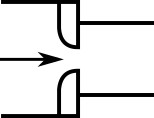
Figure 2: Round-edged orifice with different upstream and downstream pipe areas
Round-Edged Orifice with Identical Upstream and Downstream Diameters
When the upstream and downstream pipe diameters are the same for a round-edged orifice as shown in Figure 3, the round-edged orifice equation for the same pipe areas is used and is given by the following (Idelchik, 2007Idelchik, I. E., Handbook of Hydraulic Resistance, 4th edition, Begell House, Redding, CT, 2007.,262)

where

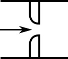
Figure 3: Round-edged orifice with the same upstream and downstream pipe areas
For other orifice configurations, see Chapter 4 of Idelchik's Handbook of Hydraulic Resistance (2007).
Discharge Coefficient Loss Model - Exit
When determining the pressure loss across the junction, xStream calculates a subsonic discharge coefficient area (CdA) for the orifice and applies the following set of isentropic compressible flow equations to solve for the static pressure and Mach number at the vena contracta


Where ṁ̇ represents the mass flow rate, To is the stagnation temperature, Po denotes the stagnation pressure, M is the Mach number, γ is the specific heat ratio, R is the gas constant, Z is the gas compressibility factor, and P is the static pressure. Note that the specific gas constant, R, is defined as the universal gas constant divided by the molecular weight of the gas.
For information on the discharge coefficient loss model see the Discharge Coefficient Loss Model topic. For information on the orifice loss when the flow is choked see the Sonic Choking description.
Discharge Coefficient Loss Model - Inline
An alternate loss model is available for inline orifices. This model differs from the exit discharge coefficient orifice model in that it includes the effect of dynamic pressure recovery that occurs in the downstream pipe, making it more appropriate for inline junctions. The mass flow through the junction is calculated via the following equation: (Perry, 10-14 (1997)Perry, R. H., Green, D. W., Perry's Chemical Engineers' Handbook, 7th Edition, McGraw-Hill, New York, NY, 1997.)

Where ṁ is the mass flow rate, Y is the expansibility factor, A is the throat area of the orifice, P1 is the inlet pressure, P2 is essentially the pressure at the vena contracta, gc is the unit conversion constant, ρ1 is the inlet density, and β is the diameter ratio of the throat relative to the upstream pipe. While this is equivalent to the flow calculation in ASME MFC-3M-2004, the two approaches differ in calculation of expansibility factors and in the conversion from the differential pressure, P1 - P2, to the irreversible pressure loss.
Note: The differential pressure loss P1 - P2 is not equivalent to the change in static pressure across the junction. The static pressure at the throat, P2, is not equal to the static pressure into the downstream pipe, which assumes fully developed flow and depends on the pipe area.
The expansibility factor, which can be viewed as a junction Output Parameter, is calculated in terms of the pressure ratio r and specific heat ratio γ.

As previously noted, the differential pressure is the pressure difference between the upstream pressure and the vena contracta, and does not account for the recovery of the dynamic pressure that occurs in the downstream pipe. Because the flow is assumed to be fully developed at the inlet of the downstream pipe, this recovery must be incorporated at the junction itself by converting the differential pressure loss to the irreversible pressure loss, which is treated as the stagnation pressure loss.

More information is available in the Discharge Coefficient Loss Model topic.