For the Metric units version of this example, click here.

Summary

A frequency analysis is performed on a system with a positive displacement compressor to determine the acoustical frequencies that need to be evaluated for the existing piping configuration.

Topics covered

• Using the PFA module to identify natural acoustic frequencies

• Defining valid sectioning and simulation duration settings for pulsation analysis

• Checking API-618 compliance

Required knowledge

This example assumes the user has already worked through the Beginner: Tank Blowdown example, or has a level of knowledge consistent with that topic.

Model file

• US - Frequency Analysis PFA.xtr

Step 1. Start AFT xStream

Open AFT xStream. Click the Start Building Model button.

From the Startup window under the "Activate Modules" section in the center panel, select the PFA (Pulsation Frequency Analysis) option to activate the PFA module. If AFT xStream is already running, choose Activate Modules from the Tools menu, then check the box next to PFA to activate the module on the Modules panel.

Step 2. Build the model

A. Place the pipes and junctions

The next step is to define the pipes and junctions. In the Workspace window, assemble the model as shown in Figure 1.

B. Enter the pipe and junction data

The system is in place but now we need to enter the input data for the pipes and junctions. Enter the following data:

All Pipes are Steel - ANSI, STD (schedule 40), and have standard roughness. The rest of the pipe information is as follows:

Pipe #	Length (feet)	Size (inches)
1	25	10
2	25	10
3	25	10
4	250	16
5	10	6

1. Assigned Flow J1

   1. Elevation = 12 feet

   2. Name = PD Compressor

   3. Mass Flow Rate =100 lbm/s

   4. Temperature = 100 deg. F

2. Valve J2

   1. Elevation =12 feet

   2. C_v = 446

   3. X_t = 0.8

3. Branch J3

   1. Elevation = 12 feet

4. Valve J4

   1. Elevation = 0 feet

   2. C_v = 1570

   3. X_t = 0.6

5. Assigned Pressure J5

   1. Elevation = 0 feet

   2. Stagnation Pressure = 0 psig

   3. Temperature = 100 deg F

6. Dead End J6

   1. Elevation = 12 feet

   2. Name = Closed Valve

C. Check if the pipe and junction data is complete

• ØTurn on List Undefined Objects from the Main Toolbar to verify if all data is entered. If it is not, the undefined pipes and junctions window will show a list of incomplete items. If there are undefined objects, go back to the incomplete pipes or junctions and enter the missing data.

Step 3. Specify Analysis Setup

A. Specify the Fluid panel

• ØOpen the Analysis Setup window and select the Fluid panel under the Fluid Properties group. Under the "AFT Standard" fluid option, choose "Methane" from the list and click the "Add to Model" button. Click OK.

B. Specify the Pipe Sectioning and Output panel

• ØOpen the Pipe Sectioning and Output panel in the Pipe Sectioning and Output group. Define the Minimum Number of Sections per Pipe as 8 sections and the Estimated Maximum Pipe Temperature During Transient as 150 deg. F.

C. Specify the Simulation Mode/Duration panel

• ØOpen the Simulation Mode/Duration panel in the Transient Control group. Enter the Stop Time as 2 seconds.

D. Specify the Pulse Setup panel

• ØOpen the Pulse Setup panel from the Pulsation Setup group. The Pulse Setup panel is used to specify the location and magnitude of the pulse applied to the system, as well as the parameters required to generate the forcing function for frequency analysis.

Define the Pulsation inputs as follows (Figure 2):

1. Check that junction J1 is selected for the pulse to be applied at. Note that the pulse may only be applied at Assigned Flow or Compressor junctions.

2. For Magnitude, ensure that Automatic (Twice Steady-State Flow) is selected.

3. Under Frequency Analysis, define the Cutoff Frequency as 200 Hz and verify that the Minimum Number of Frequency Samples is set to the default value of 1000.

4. Leave the Evaluate with API-618 option unchecked. This option will be used in a later step once the acoustic frequencies have been determined.

Now that all of the pulsation inputs are defined, look at the Pulsation Summary at the bottom of the window. The defined Cutoff Frequency and the Minimum Number of Frequency Samples will affect the number of sections and the simulation duration that are required to run the analysis. If the number of sections is insufficient, then the time step will be too large to capture the specified Cutoff Frequency. Similarly, if the simulation duration is too small, then the number of time steps will not accommodate the Minimum Number of Frequency Samples.

Checking the Pulsation Summary for this example, the Minimum Sections Required for Cutoff are 2, and the Minimum Simulation Duration Required for Min. Samples is 0.80 seconds. Both of these requirements are satisfied by the current model settings. The "Update For Me" button can be used to automatically change the minimum number of sections and/or the minimum simulation duration if they are insufficient. Click OK to exit the Analysis Setup window.

Step 4. Run the model

• ØSelect "Run Model" from the Main Toolbar. This will open the Solution Progress window. This model has an estimated run time of 5 minutes, but the run time is dependent on the speed of your PC.

Step 5. Review the frequency results

• ØOpen the Graph Results window. The first step will be to generate a plot of the pressure in each of the pipes to ensure that the simulation duration was long enough for the response to stabilize. Create the pressure graph as follows:

1. Select the Transient Pipe tab in the Graph Control tab in the Quick Access Panel

2. Add the inlet and outlet station for each of the pipes

3. Under Select Parameter choose "Pressure Static" and verify "psia" are the selected units

4. Click Generate

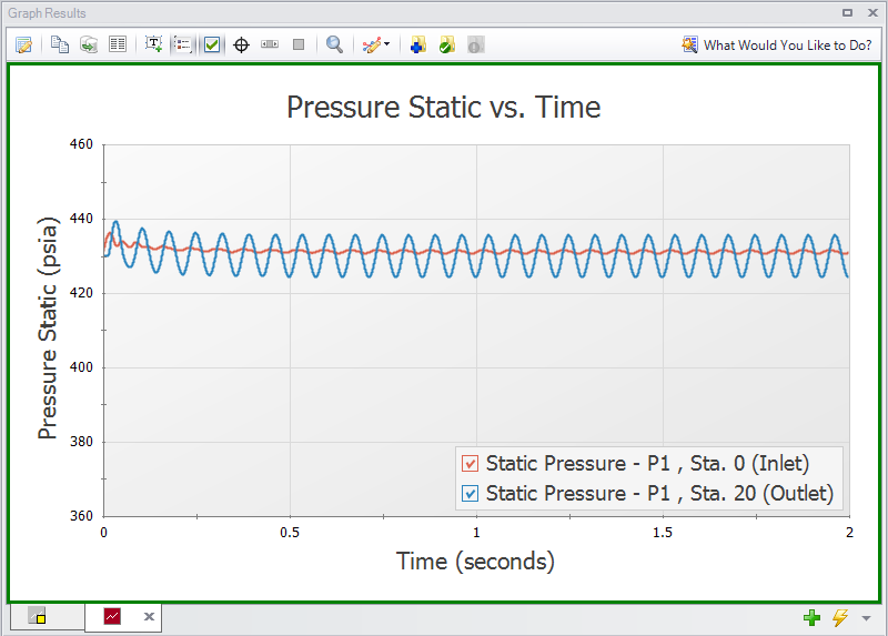
The pressure graph should appear as shown in Figure 3. Note that there is a small perturbation in the pressure when the pulse is applied to the system, though the pressure results completely stabilize by the end of the run. If the pressure results were still changing at the end of the run, the model should be re-run with a longer simulation duration.

Next, graph the acoustic frequency response as follows:

1. Click the "New Tab" button

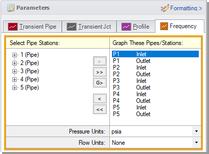
2. Select the Frequency tab in the Graph Parameter section of the Quick Access Panel (Figure 4)

3. Add the inlet and outlet station for each of the pipes

4. Verify that the pressure units are set to psia

5. Click Generate

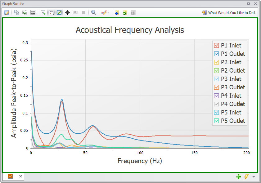
Identify excitation frequencies to study

From the graph in Figure 5, there are several frequencies that produce a large pressure response. Points on the plot with a large response magnitude are easily identified by finding local maxima on the graph. These maxima are the acoustic natural frequencies that are potentially the most damaging when excited by a positive displacement compressor. These frequencies can also be caused by equipment that contributes large pressure drops, such as control valves.

Two natural frequencies are identified for the system based on the peaks in the graph at roughly 28 Hz and 57 Hz. Note that the number of sections used for the analysis may affect the location of the peaks, so it is prudent to run the analysis with more sections to reduce uncertainty in the results. It is also recommended to analyze frequencies near identified peaks (for example, analyzing 55 and 59 Hz for the peak at 57 Hz) to account for potential shifting of the frequency peaks that can result from the assumptions made for the frequency analysis in AFT xStream.

Step 6. Determine the pressure response for API-618

The identified excitation frequencies can now be used to determine the pressure response in the system caused by the pulsation at the compressor. The pressure response can then be evaluated for compliance with API-618.

To determine the pressure response of the excitation frequencies, complete the following steps:

1. In the Scenario Manager, right-click on the base scenario and choose "Create Child". Name the child scenario "28 Hz".

2. Open the Analysis Setup window and go to the Pulse Setup panel.

3. Check the box to "Evaluate with API-618 and enter the Speed as 750 rpm and the Number of Heads as 2.

4. Enter the Time Until Steady State Pulsation as 0.25 seconds. The method to find this value is discussed later in the example. Click OK to close Analysis Setup.

5. Open the Assigned Flow Properties window for junction J1.

6. In the Transient tab, clear the pulse transient data by clicking Edit Table under the transient table and choosing Clear All Data.

7. Check the box next to Periodic Flow. Define the Frequency as 28 1/s and the Flow Amplitude as 10 lbm/sec (Figure 6).

8. Click OK to close the Properties window.

The model is now updated to represent the pulsation at the positive displacement compressor that will excite the system. Run the model, then navigate to the Output window. This scenario will run faster than the base scenario (about 2 minutes).

In the Output window there is now a warning stating that the maximum pressure limit for API-618 was exceeded as is shown in Figure 7. When the API-618 evaluation is performed the Pulsation Summary tab is shown in the Output window with additional information on where pressure limit violations occurred, and what inputs were used to calculate the API-618 pressure limits for the scenario (Figure 8).

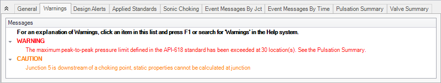
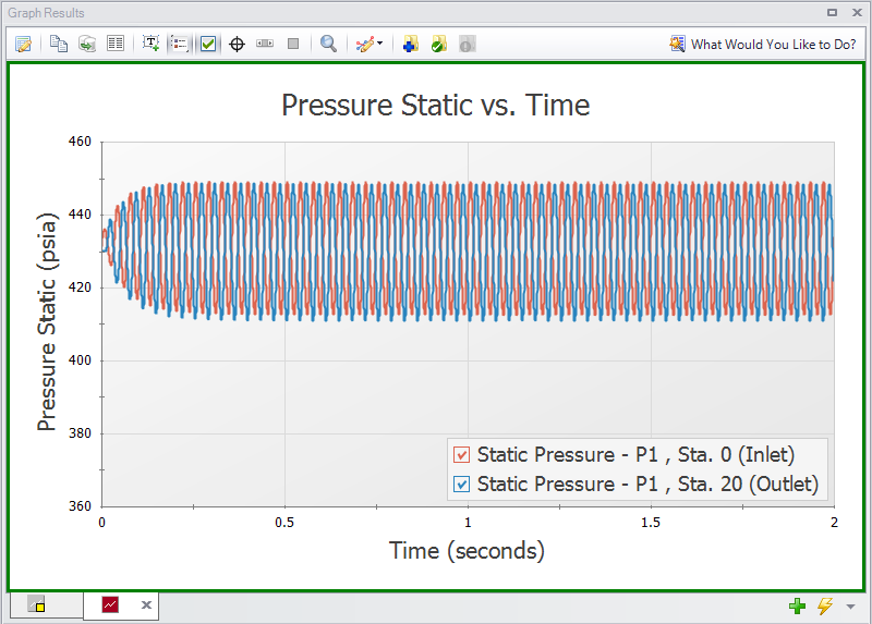
In the Graph Results window, generate a graph of the static pressure following the same process used to create Figure 3. However, only include the pipe P1 inlet and outlet station. The resulting graph is shown in Figure 9. These pressure results can be used to check for compliance with standards such as API-618.

The pressure results for the compressor outlet (Pipe P1 inlet) can also be used to determine the Time Until Steady State Pulsation, which is one of the inputs needed to accurately evaluate API-618. The Time Until Steady State Pulsation is the time at which the pressure oscillations have a consistent amplitude. In Figure 9 below the wave heights appear to become consistent at about 0.25 seconds.

Note for this example the value of 0.25 seconds was given in advance to expedite the process, but normally the user would need to run the model once with the "Time Until Steady..." set to 0, then determine the time input and re-run the model with the correct value.

For comparison, this model can also be run at one of the frequencies which gave a lower amplitude, such as 14 Hz. At 14 Hz, a lower amplitude pressure response is produced, as can be seen in Figure 10.

Note: The pulsation observed in this model represents a pure sine wave. Real systems might have a different forcing function.

Conclusion

The PFA add-on module for AFT xStream can be used to apply a pressure pulse to the system in order to identify acoustic frequencies which may result in damage. These frequencies can be used in further pulsation analysis to determine if pulsation mitigation is required, and what mitigation would be effective.