High Pressure Steam - Forces Example (English Units)
For the Metric units version of this example. click here.
Summary
Two turbines in a high pressure steam system are simultaneously valved off, which causes the system to experience transient forces. This example describes how to determine the imbalanced transient force data for the piping system during the steam flow transient. It also evaluates the effect of varying the time to close the valves on force magnitude. Lastly, this example shows how to export the force results to a force file to use in piping stress software.
Topics covered
-
Calculating the forces associated with a transient event
-
Using the Scenario Comparison Tool to compare scenarios
-
Exporting force sets to CAESAR II®
Required knowledge
This example assumes the user has already worked through the Beginner: Tank Blowdown example, or has a level of knowledge consistent with that topic.
Model file
If this example is being completed as part of the Quick Start, the partially completed model can be downloaded from the link below
Step 1. Start AFT xStream
Open AFT xStream. Click the Start Building Model button.
Step 2. Build the model
A. Place the pipes and junctions
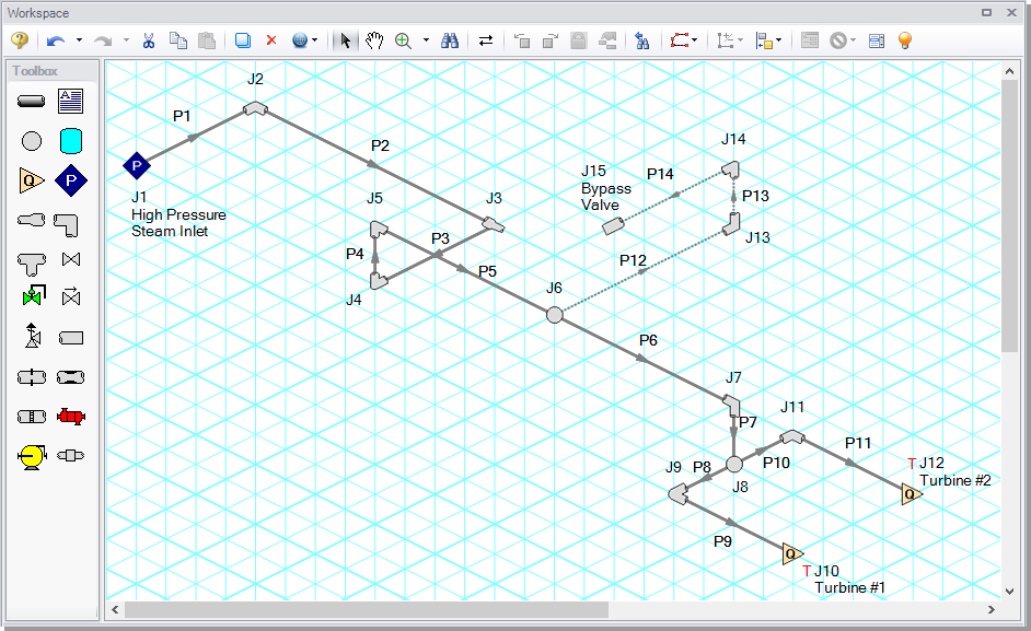
This example will be created in the isometric view in order to get a greater feel for the pipe layout.
-
Open the Arrange menu again and select the Isometric option under Pipe Drawing Mode
-
Place the junctions as shown in Figure 1
-
Click the pipe tool and draw the pipes in the model as shown
-
Use the Rotate Icons button, or right click on the junction and select Auto-rotate Icon to align the junction with the connected pipes. Alternatively, the Customize Icon option can be selected from the right-click menu to manually choose an icon/orientation.
-
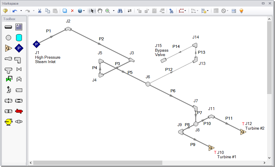
The grid can be shown or turned off in the Arrange menu, as shown in Figure 2
Note: You can hold the "Alt" key while adjusting a pipe by the endpoint to add an additional segment . This can be used with the arrow key or mouse scroll wheel to change between different preview line options.
B. Enter the pipe data
The system is in place, but now the input data for the pipes and junctions needs to be entered. Double-click each pipe or junction and enter the following data in the Pipe or Junction Properties windows.
All pipes in the model are User Specified and utilize a User Specified Friction Model with an Absolute Roughness of
| Pipe | Internal Diameter (inches) | Length (feet) |
|---|---|---|
| 1 | 13.2 | 13 |
| 2 | 13.2 | 40 |
| 3 | 10.6 | 13 |
| 4 | 10.6 | 13 |
| 5 | 10.6 | 33 |
| 6 | 10.6 | 43 |
| 7 | 10.6 | 6.5 |
| 8 | 10.6 | 5 |
| 9 | 8.1 | 20 |
| 10 | 10.6 | 5 |
| 11 | 8.1 | 20 |
| 12 | 6.5 | 50 |
| 13 | 6.5 | 10 |
| 14 | 6.5 | 10 |
C. Enter the junction data
-
Assigned Pressure J1
-
Name = High Pressure Steam Inlet
-
Elevation = 0
-
Static Pressure =
-
Static Temperature =
-
-
Bend J2, J4
-
Elevation = 0
-
Type = Standard Elbow (knee, threaded)
-
-
Area Change J3
-
Elevation = 0
-
Type = "Conical Transition"
-
Angle = 45 degrees
-
-
Bend J5, J7, J13
-
Elevation =
-
Type = Standard Elbow (knee, threaded)
-
-
Branch J6
-
Elevation =
-
-
Branch J8
-
Elevation =
-
-
Bend J9, J11
-
Elevation =
-
Type = Standard Elbow (knee, threaded)
-
-
Assigned Flow J10, J12
-
J10 Name = Turbine #1
-
J12 Name = Turbine #2
-
Elevation =
-
Mass Flow Rate =
-
Temperature =
-
On the Transient tab enter the following data for both Assigned Flow junctions:
-
| Time (seconds) | Mass Flow Rate ( |
Static Temperature (deg. |
|---|---|---|
| 0 |
|
|
| 0.1 | 0 |
|
| 1 | 0 |
|
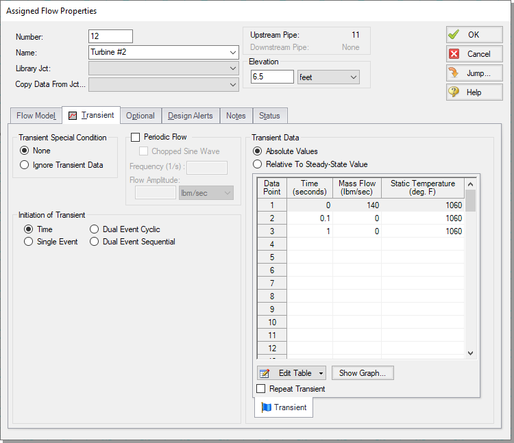
Figure 3: Transient data for Assigned Flow junctions J10 and J12
-
Bend J14
-
Elevation =
-
Type = Standard Elbow (knee, threaded)
-
-
Dead End J15
-
Name = Bypass Valve
-
Elevation =
-
D. Check if the pipes and junctions are specified
-
ØClick the List Undefined Objects button to see if the model is fully defined. If it is not, the undefined pipes and junctions window will show a list of incomplete items. If undefined objects are present, go back to the incomplete pipes or junctions and enter the missing data.
Step 3. Specify Fluid
-
ØSelect Fluid from the Analysis menu to open the Fluid panel in the Analysis Setup window. For this example, select the AFT Standard fluid option, then choose "Steam" from the list and click the "Add to Model" button.
Step 4. Specify the Pipe Sectioning and Output panel
-
ØOpen the Pipe Sectioning and Output panel in the Analysis Setup window. Define the Minimum Number of Sections Per Pipe as 1 section and the Estimated Maximum Pipe Temperature During Transient as

Step 5. Specify the Simulation Mode/Duration panel
-
ØOpen the Simulation Mode/Duration panel from the Transient Control group. Enter the Stop Time as 1 second. Click OK to close the Analysis Setup window.
We will first add one Force Set from the Workspace.
-
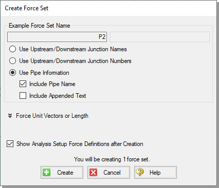
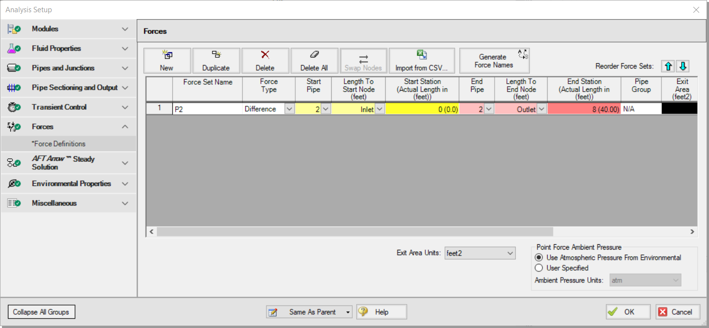
ØOn the Workspace, right-click on pipe P2 and from the right-click menu select "Create a Force Set with Selected Pipe." Select the Use Pipe Information radio button and uncheck the "Include Appended Text" option (Figure 5). Click Create. This will open the Force Definitions panel of the Analysis Setup window. The Force Definitions panel should appear as shown in Figure 6.
AFT xStream can only determine axial forces down a pipe in the direction defined as forward by the force set definition. As such, AFT xStream has no knowledge of the three-dimensional orientation of a given force set. For example, a vertical pipe and a horizontal pipe that both have the same force magnitude would be indistinguishable in AFT xStream. The force set definition informs the sign of the force, with a positive value indicating a force pushing from the start location to the end location, and a negative value indicating the converse.
If a more robust view of the 3D orientation of the pipes is required, directional information can be entered using the optional Force Unit Vector columns. The Force Unit Vectors do not impact AFT xStream's calculations, but may be useful to export the output to piping stress analysis software as discussed in Step 12
Note: Only single pipes can be added as a "Difference" force set type from the Workspace. Also note that difference forces should strictly be used between two 90 degree angle pipe fittings.
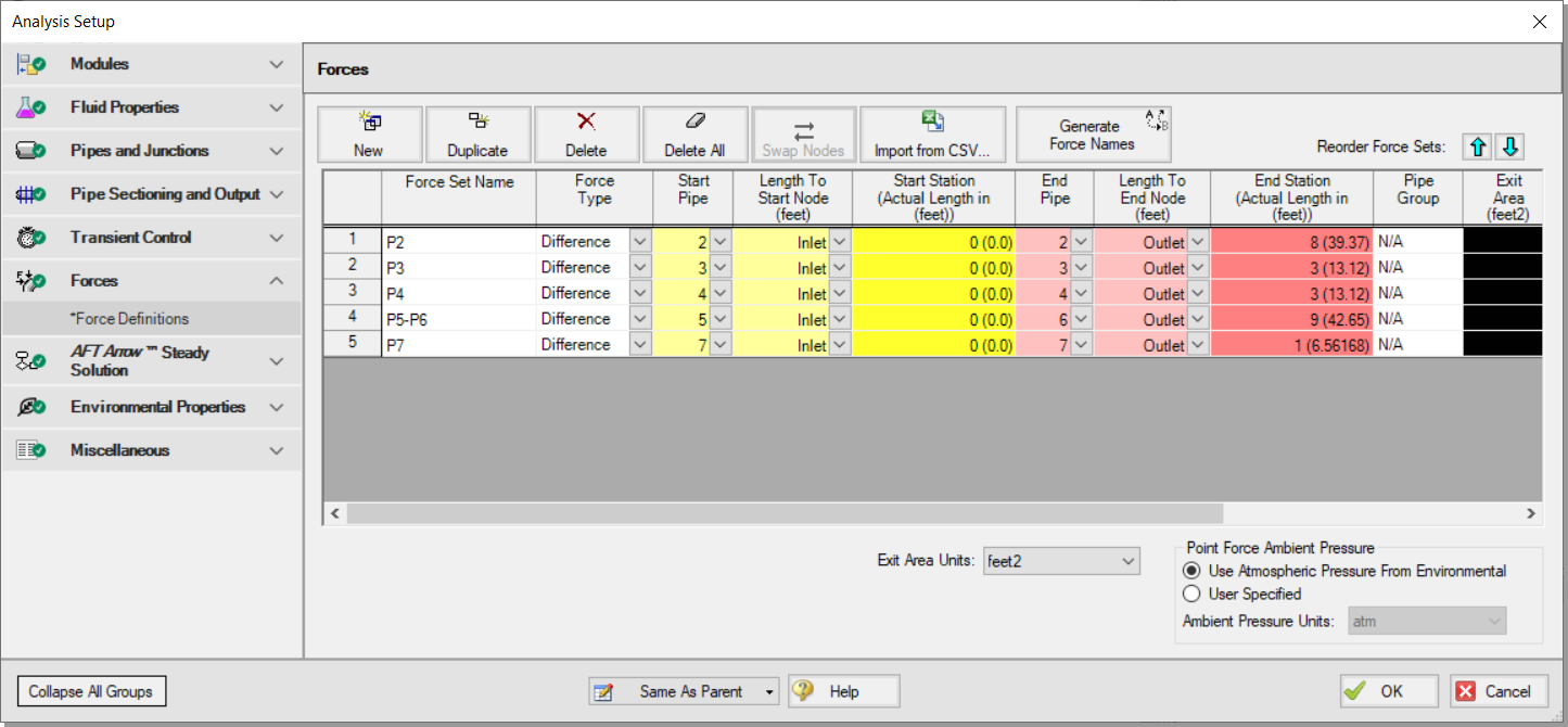
The remaining force sets will be defined inside the Force Definitions panel.
-
ØDefine a force set by clicking "New", selecting the Force Type (in this example, we will be using "Difference"), entering a name, and defining the starting and ending locations of the force set. Set up the force sets as shown in Figure 7. Click OK to exit the Analysis Setup window.
Step 7. Add child scenarios using Scenario Manager
A. Create scenarios
In this model, we will evaluate three different valve closure durations for the system:
-
0.1 Second Valve Closure
-
0.25 Second Valve Closure
-
0.5 Second Valve Closure
We will create three child scenarios to model the three cases.
-
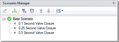
ØGo to the Scenario Manager on the Quick Access Panel. Create a child scenario by either right-clicking on the Base Scenario and then selecting Create Child
 . Enter the name "0.1 Second Valve Closure" in the Create Child Scenario window, and click OK. The new "0.1 Second Valve Closure" scenario should now appear in the Scenario Manager on the Quick Access Panel below the Base Scenario.
-
ØRight-click the Base Scenario in the Quick Access Panel. Create another child and call it "0.25 Second Valve Closure". Finally, create one more child and call it "0.5 Second Valve Closure". The child scenarios should now be displayed as shown in Figure 8.
B. Define the child scenarios
Since the "0.1 Second Valve Closure" scenario uses the same transient definitions as the base scenario, we do not need to modify it. We will set up the remaining scenarios using the following steps:
-
Open the "0.25 Second Valve Closure" scenario by double-clicking the name in the Scenario Manager
-
Open the Assigned Flow Properties window for Assigned Flow J10 and open the Transient tab. Enter the following data:
| Time (seconds) | Mass Flow( |
Static Temperature (deg. |
|---|---|---|
| 0 |
|
|
| 0.25 | 0 |
|
| 1 | 0 |
|
-
Enter the same Transient Data for Assigned Flow J12
-
Open the Child Scenario "0.5 Second Valve Closure" from the Scenario Manager
-
Open the Assigned Flow Properties window for Assigned Flow J10 and open the Transient tab. Enter the following data:
| Time (seconds) | Mass Flow( |
Static Temperature (deg. |
|---|---|---|
| 0 |
|
|
| 0.5 | 0 |
|
| 1 | 0 |
|
-
Enter the same Transient Data for Assigned Flow J12
Step 8. Compare child scenarios using the Scenario Comparison Tool
The three scenarios created should be identical except for the different transient data. To confirm the scenarios are otherwise identical, we will use the Scenario Comparison Tool.
-
Load the "0.1 Second Valve Closure" scenario from the Scenario Manager
-
In the Tools menu, select the Scenario Comparison Tool
-
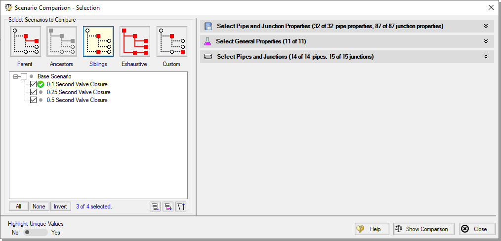
In the Scenario Comparison - Selection window (Figure 9), select "Siblings"
-
Click "Show Comparison"
-
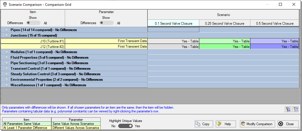
In the Scenario Comparison Grid, set the "Item" and "Parameter" sliders to show "Differences". Also set the "Highlight Unique Values" slider to "Yes".
The Scenario Comparison Tool will run a comparison of all Pipe and Junction Properties as well as the General Properties used in each scenario and highlight any differences in the Scenario Comparison Grid. In this model, the only highlighted differences should be for the "First Transient Data" parameter for junctions J10 and J12 (Figure 10). Note that each column in the Scenario Comparison Grid is highlighted in a different color. This indicates that each scenario possesses a unique value for the given parameters. Click close to exit the Scenario Comparison Tool.
Step 9. Run the first scenario
-
ØDouble-click the "0.1 Second Valve Closure" child scenario in the Scenario Manager. Ensure that all force sets are set to be applied in the Force Definitions panel of the Analysis Setup window as shown in Figure 7. Select "Run Model" from the Analysis menu. This will open the Solution Progress window. This model has an estimated run time of 1 minute, but the run time is dependent on the speed of your computer.
Step 10. View the results
-
ØIn the Output window, click on the Forces tab. This will show the maximum force observed in the defined force sets, as well as provide information about how the force segments were defined.

Figure 11: Forces tab in the Output window for the "0.1 Second Valve Closure" scenario
B. Graph the force results
-
ØOpen the Graph Results window. We will create a graph that shows the transient forces over time for the force sets. To do so, perform the following steps:
-
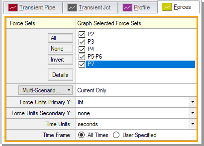
Select the Forces tab on the Graph Control tab on the Quick Access Panel, as shown in Figure 12.
-
Select "All" force sets to be graphed.
-
Verify the Force Units Primary Y is set to "
-
Verify that Time Units is set to "seconds."
-
Verify that the Time Frame is set to "All times."
-
Click Generate.
This should generate the graph shown in Figure 13.
Add the graph to the Graph List Manager by right-clicking the graph results window and selecting "Add Graph To List...". Name the graph "Force Sets" and click OK.
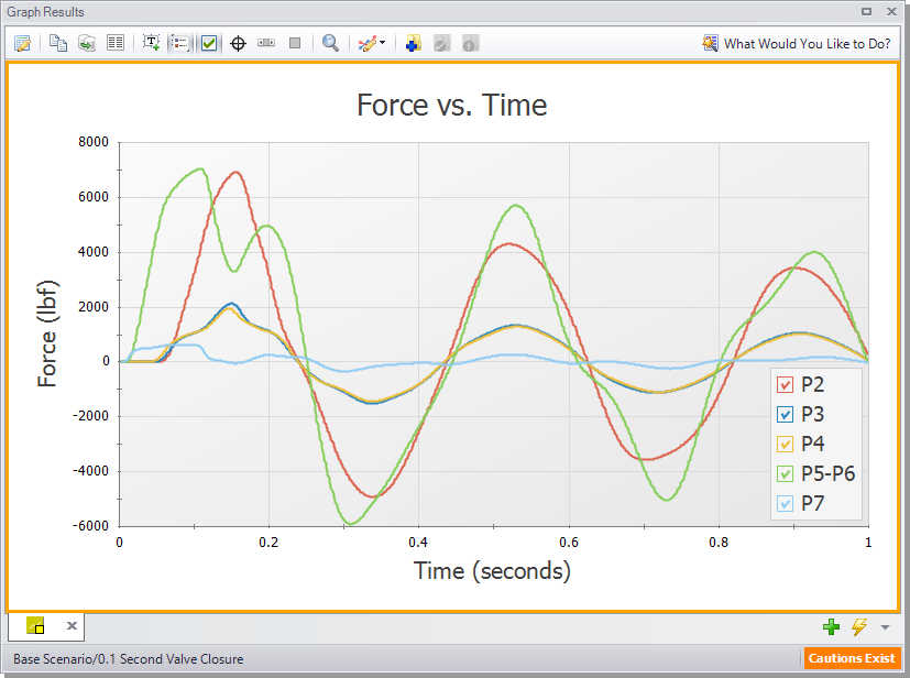
Note that at t = 0 seconds, there are no force imbalances for any of the force sets. This is expected since the sum of forces across a piping run between two elbows equals zero in a steady state system. If a Point or Exit type force set were used instead of a Difference type force set, then a non-zero force may be encountered during the steady state.
Additionally, some traditional methods of analyzing force sets will not yield the same results as AFT xStream since they may not include friction or momentum effects in their force balances. Traditional methods can yield significantly different results and indicate incorrect, non-zero forces during steady state conditions.
There are two important points to be observed here:
-
AFT xStream calculates transient fluid forces. This does not include piping, component, or fluid weight, or any other forces external to the piping. A comprehensive analysis of pipe loading must separately include these items.
-
Ignoring friction and momentum force balance components will result in force imbalances that do not exist.
Step 11. Run the other child scenarios
-
ØRun the other two child scenarios and load the Forces tab and the "Force Sets" graph list item for each. The results are seen below in Figures
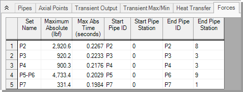
Figure 14: Forces tab in the Output window for "0.25 Second Valve Closure" scenario
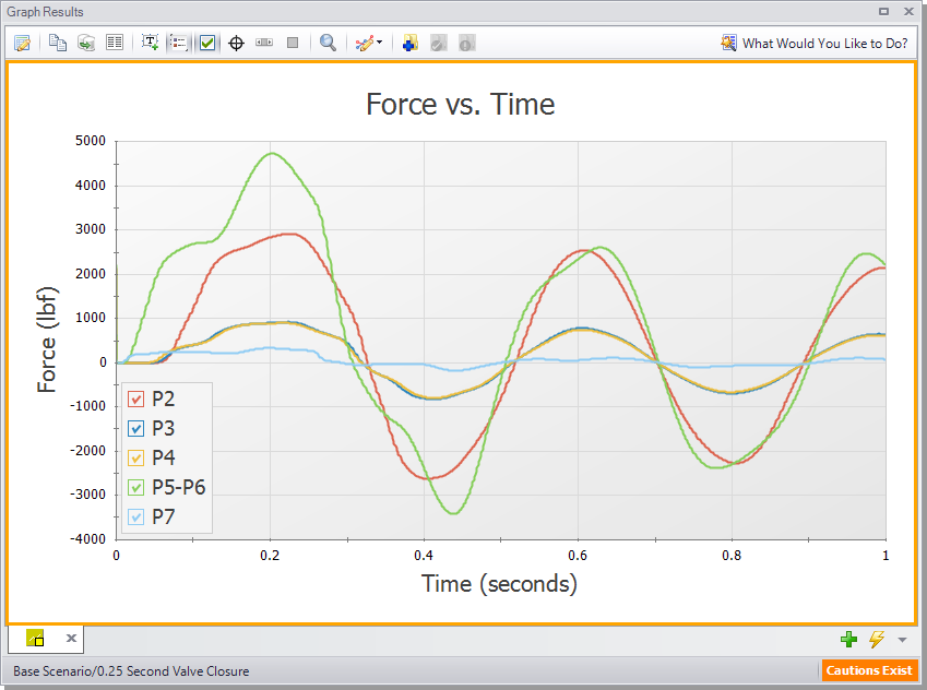
Figure 15: Graph for forces of the "0.25 Second Valve Closure" scenario
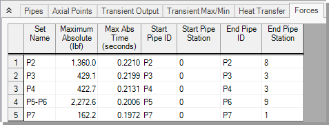
Figure 16: Forces tab in the Output window for the "0.5 Second Valve Closure" scenario
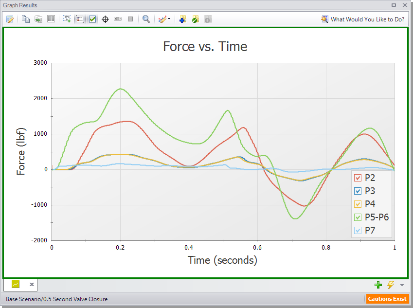
Figure 17: Graph for forces of the "0.5 Second Valve Closure" scenario
These figures show that the maximum force magnitude increases as the valve closes faster. Typically, the more rapidly a change occurs, the more severe the resulting forces are. Therefore, a utility of AFT xStream would be to evaluate the correlation between transient event duration (e.g., valve closing time) and the resultant force magnitudes.
Factors affecting the timing and magnitude of forces
Pipe sectioning, the selection of fluid property model, and specification of Maximum Pipe Mach Number During Transient can have a significant effect on the accuracy of the forces calculated by AFT xStream. This effect was not significant in the system built within this example. However, the results for altering each of these three parameters are shown in Figures
If you wish to learn more about the effect of altering these 3 factors with regards to force, the click here to go to the Transient Sensitivity Analysis Tutorial.
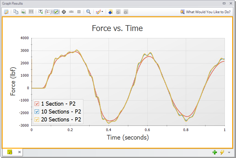
Figure 18: Effect of sectioning on High Pressure Steam - Forces model. All runs use the AFT Standard fluid library and a Maximum Pipe Mach Number During Transient of 1.

Figure 19: Effect of fluid property model on High Pressure Steam - Forces model. All runs use a Minimum Number of Sections Per Pipe of 1 and an Estimated Maximum Pipe Mach Number During Transient of 1.

Figure 20: Effect of Maximum Pipe Mach Number During Transient on High Pressure Steam - Forces model. All runs use the AFT Standard fluid library.
Step 12. Export CAESAR II Force file
-
ØOpen the Output window, and click on the File menu. Select "Export Force File..." and choose "CAESAR II® Force File." This will open the export file window shown in Figure 21.
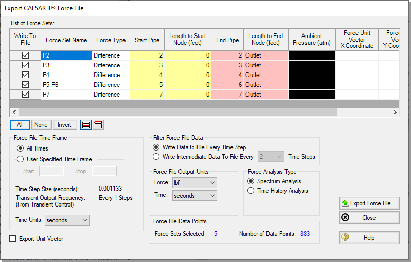
The force sets to include in the force file may be individually selected, along with how frequently data points are saved. The number of data points that will be in the file is also displayed for the given setting. This number should not exceed the maximum number of data points allowed for the relevant piping stress software, which in the case of CAESAR II® is 2500.
If unit vector information has been entered in the Force Definitions panel, the Export Unit Vector option can be used to include this information in the exported file. Similar methods to those described above can be used to export force files to ROHR2®, TRIFLEX®, and AutoPIPE®.
Conclusion
We created a force model to calculate the forces experienced as a result of two simultaneous closures in a steam header. We also identified how the length of the transient can have a significant impact on the forces a system experiences. Finally, we discussed how to export these forces into a force file to be used in pipe stress analysis software.