Gas Turbine Fuel System Example (English Units)
For the Metric units version of this example, click here.
Summary
A compressor feeding natural gas to combustion baskets in a Turbine Fuel System has one of its 3 control valves close instantaneously. The effect of this transient event on the temperature, pressure, and velocity of the system is observed.
Topics covered
This example will cover the following topics:
-
Modeling a valve closure as a transient event
-
Modeling a heat exchanger
-
Using the Scenario Manager in AFT xStream
-
Indicating the importance of the Estimated Maximum Temperature During Transient
-
Creating animated profile graphs
Required knowledge
This example assumes the user has already worked through the Beginner: Tank Blowdown example, or has a level of knowledge consistent with that topic.
Model file
Step 1. Start AFT xStream
Open AFT xStream. Click "Start Building Model".
Step 2. Build the model
A. Place the pipes and junctions
The first step is to define the pipes and junctions. In the Workspace window, assemble the model as shown in Figure 1.

B. Enter the pipe and junction data
The system is in place but now the input data for the pipes and junctions needs to be entered. Enter the following data in each Pipe and Junction Properties window.
All Pipes are Stainless Steel - ANSI, Schedule 10S, and have standard roughness. The rest of the pipe information is as follows:
| Pipe # | Size (inches) | Length (feet) |
|---|---|---|
| 1 | 8 | 75 |
| 2 | 8 | 25 |
| 3 | 8 | 5 |
| 4 | 5 | 5 |
| 5 | 5 | 5 |
| 6 | 8 | 5 |
| 7 | 5 | 5 |
| 8 | 5 | 5 |
| 9 | 8 | 5 |
| 10 | 5 | 5 |
| 11 | 5 | 5 |
Because several of the pipes are the same, you can use the Global Pipe Editing tool to speed up the process of entering the data. The Global Pipe Editing tool allows you to apply changes to multiple pipes at the same time. Select Global Pipe Edit either from the Edit Menu, or by selecting the "Global Edit" dropdown on the toolbar and selecting the "Global Pipe Edit" option. This will open the Global Pipe Edit window. Select pipes P4, P5, P7, P8, P10, and P11 from the list of pipes as shown in Figure 2.

After selecting the pipes, click the "Select Pipe Data" button. This will open a template Pipe Properties window for entering the data to be applied to all of the selected pipes. Fill out the data for the selected pipes. When you have entered all of the data for the pipes, close the Pipe Properties window by selecting OK. The Global Pipe Edit window will now display a list of all of the parameters that may be applied to the selected pipes. The parameters are categorized as they are displayed on the tabs in the Pipe Properties window. For this example, you want all of the parameters for all of the selected pipes to be updated to the specified values. This can be accomplished by selecting the "All" button above the list of parameters. The Global Pipe Edit window should now appear as shown in Figure 3.
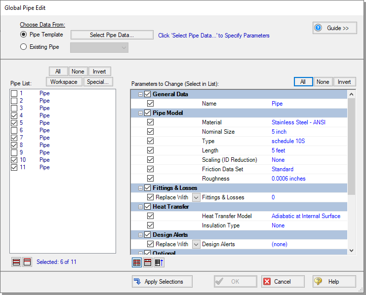
Apply the changes to the selected pipes by clicking the "Apply Selections" button. AFT xStream will notify you that the changes have been completed. Select OK. At this point, all of the changes have been applied but not saved. If you wish to cancel all of the changes you just implemented, you may do so by clicking Cancel on the Global Pipe Edit window. Save the applied changes by clicking OK.
Notes: The "Guide >>" button in the Global Edit windows may be used as a reminder of the required steps for the global edit process if needed.
-
Assigned Flow J1
-
Name = PD Compressor
-
Elevation =
-
Mass Flow Rate =
Note: Be advised that the unit for mass flow is not the default as it is
-
Temperature =
-
-
Heat Exchanger J2
-
Name = Natural Gas Heater
-
Elevation =
-
K = 6.6
-
Steady Heat Rate =
Note: Be advised that the unit for heat rate is not the default as it is Btu/hr as opposed to Btu/s.
-
-
Valve J3
-
Elevation =
-
Cv = 10,000
-
Xt = 0.3
-
-
Valve J5
-
Name = Diffusion Gas FCV
-
Elevation =
-
Cv = 95
-
Xt = 0.7
-
-
Valve J8
-
Name = Premix Gas FCV #1
-
Elevation =
-
Cv = 195
-
Xt = 0.7
-
-
Valve J11
- Name = Premix Gas FCV #2
-
Elevation =
-
Cv = 195
-
Xt = 0.7
-
Click on the Transient Tab and enter the following data
| Time (seconds) | Cv | Xt |
|---|---|---|
| 0 | 195 | 0.7 |
| 0.01 | 0 | 0.7 |
| 2 | 0 | 0.7 |
-
Assigned Pressures J6, J9, J12
-
J6 Name = Combustion Basket #1
-
J9 Name = Combustion Basket #2
-
J12 Name = Combustion Basket #3
-
Elevation =
-
Stagnation Pressure =
-
Temperature =
-
-
Junctions J4, J7, J10
-
Elevation =
-
C. Check if the pipe and junction data is complete
-
ØOpen the List Undefined Objects window from the View Menu or the Workspace Toolbar
 to verify if all pipes and junctions are specified. If not, the incomplete pipes or junctions will be listed. If undefined objects are present, go back to the incomplete pipes or junctions and enter the missing data.
Step 3. Specify Analysis Setup
A. Specify the Fluid panel
-
ØOpen the Analysis Setup window by clicking Analysis Setup on the Main Toolbar. Under the "AFT Standard" fluid option, select "Methane" from the list and click the "Add to Model" button. Click OK.
Note: Methane is used to model natural gas in order to minimize the run time. If you need to model a real natural gas mixture, then instead of using the AFT Standard fluid library, it would be better to use the NIST REFPROP library or the optional Chempak add-on.
B. Specify the Pipe Sectioning and Output panel
-
ØOpen the Pipe Sectioning and Output panel. Set the Minimum Number of Sections Per Pipe to 8 sections and the Estimated Maximum Pipe Temperature During Transient to
Note: If following along in the completed model file, the Estimated Maximum Pipe Temperature During Transient will have a different value. This will be discussed in Steps 8 and 9.
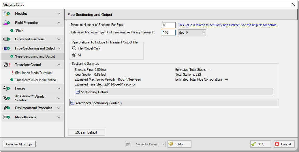
Figure 4: Sectioning panel for Turbine Fuel System
C. Specify the Simulation Mode/Duration panel
-
ØOpen the Simulation Mode/Duration panel from the Transient Control group. Enter the Stop Time as 2 seconds. Verify the Time Simulation is set to Transient. Click the OK button.
Step 4. Create scenarios to model different sectioning setups
A. Create scenarios
In this model, the following three types of Sectioning cases for the system are to be evaluated:
-
8 Sections Minimum per Pipe
-
4 Sections Minimum per Pipe
-
2 Sections Minimum per Pipe
To evaluate the three cases, we will utilize the Scenario Manager to create three scenarios for the three cases.
Open the Scenario Manager on the Quick Access Panel. Create a child scenario by either right-clicking on the Base Scenario and then selecting Create Child, or by first selecting the Base Scenario on the Scenario Manager on the Quick Access Panel and then selecting the Create Child icon .Enter the name "8 Sections Minimum Per Pipe" in the Create Child Scenario window, and select the OK button. The new "8 Sections Minimum Per Pipe" scenario should now appear in the Scenario Manager on the Quick Access Panel below the Base Scenario. Select the Base Scenario. Create another child and call it "4 Sections Minimum Per Pipe". Finally, create one more child and call it "2 Sections Minimum Per Pipe". The Child Scenarios should now be displayed as shown in Figure 5.

Figure 5: The Scenario Manager on the Quick Access Panel displays the scenario tree which allows you to create scenarios and keep them organized within the same model file
B. Set up scenarios
Since the "8 Sections Minimum Per Pipe" scenario has the same setup as the Base Scenario, we do not need to modify it. Select the "4 Sections Minimum Per Pipe" scenario by double-clicking the name in the Scenario Manager.
-
ØOpen the Analysis Setup window from the Main Toolbar. Click on the Pipe Sectioning and Output panel and change the Minimum Number of Sections Per Pipe to 4 then click OK.
ØOpen the Child Scenario "2 Sections Minimum per Pipe". Open the Analysis Setup window from the Main Toolbar. Open the Pipe Sectioning and Output panel and change the Minimum Number of Sections Per Pipe to 2 then click OK.
Step 5. Run the first scenario
-
ØDouble-click the "2 Sections Minimum Per Pipe" scenario in the Scenario Manager. Select "Run Model" on the toolbar. AFT xStream will prompt you to save, then will open the Solution Progress window. This model is estimated to run in approximately one minute, but the run time is dependent on the speed of your computer.
Step 6. Review the results
-
ØClick the Output button. This will take you to the Output window, which will display any warnings if they exist. There should be a warning indicating that the maximum transient pipe temperature was higher than the estimate as well as a caution that the maximum transient pipe mach number was significantly lower than the estimate (see Figure 6). The Estimated Maximum Pipe Temperature During Transient is critical to the calculation of transient conditions due to its necessity in the Method of Characteristics.
The Estimated Maximum Pipe Temperature During Transient is used to calculate the sonic velocity of the fluid, which is then used to create the upper boundary of the characteristic grid. If the maximum temperature during the transient exceeds the specified Estimated Maximum Pipe Temperature During Transient and the flow is sonic, the Method of Characteristics may have to extrapolate data, which can lead to instability and will stop the transient solver. In this model, sonic velocity was not reached when the temperature was higher than the estimated maximum. However, to ensure that this model can handle sonic flow, we will re-run the model with a higher Estimated Maximum Pipe Temperature During Transient.
The Maximum Transient Pipe Mach Number error indicates that error could be introduced through having a Mach Number substantially lower than the Maximum Transient Pipe Mach Number used for the calculation (in this case, the xStream default value of one). This caution will be ignored in this example for simplicity.
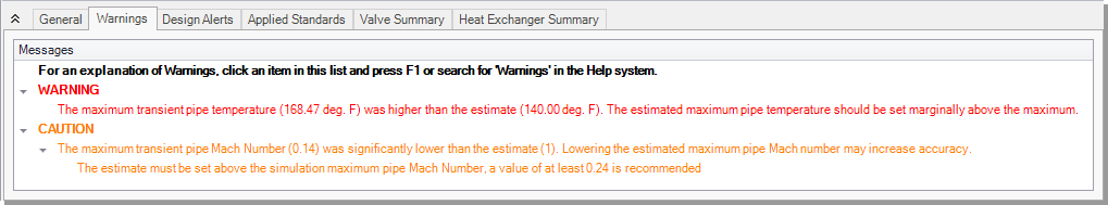
Figure 6: The maximum transient pipe temperature exceeds estimated maximum temperature warning indicates that the model is at risk of instability if changes are made
Step 7. Adjust the Pipe Sectioning panel
-
ØDouble-click "Base Scenario" in the Scenario Manager. Open the Analysis Setup window from the Main Toolbar and select the Pipe Sectioning and Output panel. Change the Estimated Maximum Pipe Temperature During Transient to
Note: It is essential that this change is made in the Base Scenario so all scenarios are updated.
Step 8. Re-run the model and review results
A. Review Output window
-
ØDouble-click the "8 Sections Minimum Per Pipe" scenario. Select "Run Model" from the Analysis menu, then proceed to the Output window. There should be a caution indicating that the maximum transient pipe mach number was significantly lower than the estimate. Disregard this error as discussed previously. Select the Transient Max/Min tab (Figure 7). Here we can see that the maximum temperature in the inlet lines (P5, P8, & P11) to the combustion baskets is
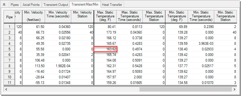
Figure 7: Transient Max/Min tab in the Output window
B. Graph the results
Go to the Graph Results window by clicking on the Graph Results tab or pressing Ctrl+G on the keyboard.
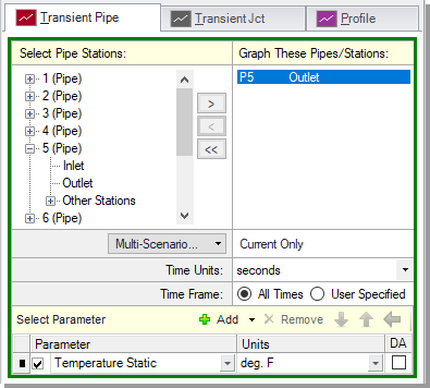
Create a graph that shows the temperature over time at the entrance to Combustion Basket #1 using the following steps:
-
From the Graph Control tab on the Quick Access Panel, select the Transient Pipe tab
-
Select Pipe P5 and add the outlet station
-
Verify that the time units are set to seconds
-
In the Parameters definition area, select "Temperature Static" and specify "deg.
-
Click the Generate button
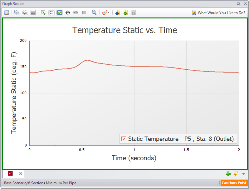
The results (see Figure 9) show a maximum temperature of
To easily recreate this graph in the other scenarios or in the future, it can be added into the Graph List Manager on the Quick Access Panel. After generating the graph, click the "Add Graph to List" icon on the Graph Results Toolbar (or simply right-click the graph itself and choose "Add Graph to List"). Give the graph a name, such as "Combustion Basket #1 Temperature vs Time", then click OK. The graph will be added to the currently selected folder in the Graph List Manager. Note that graphs added to the Graph List Manager are not permanently saved until the model is saved again. Also be aware that only the graph templates are saved as opposed to the graph data.
C. Animate the results
We will create a graph that models the temperature, pressure, and velocity along the flow path between the positive displacement compressor and Combustion Basket #1. To do this:
-
Create a new graph tab by clicking the "New Tab" button
-
Select the Profile tab under the Graph Control tab in the Quick Access Panel. Alternatively, you can access the Select Graph Parameters window by clicking on the "Select Graph Parameters" icon located at the top left of the Graph Results window.
-
Select pipes 1, 2, 3, 4, and 5
-
Select the option to Animate Using Output.
-
Ensure that the animation time used is seconds.
-
Select Temperature Static as a parameter.
-
Add Pressure Static and Velocity Parameters to the Parameters Window.
-
Click Generate.
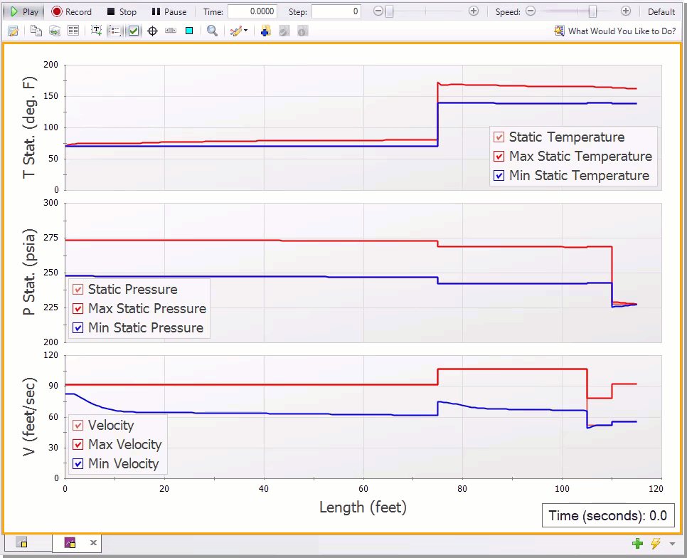
You should generate a graph that looks like the one shown in Figure 10. Playing the animation reveals that the highest temperature in the system is observed at the J2 heat exchanger. It should also be noted that the rise to this maximum temperature occurs when the pressure wave from the valve closing passes through this junction. This heightened temperature is not immediately seen by the combustion baskets downstream, however, as the gas velocity throughout the system drops immediately following the valve closure. Instead, the heightened temperature moves slowly downstream until the gas wave is reflected at the positive displacement compressor and passes through the heat exchanger going the opposite direction. This causes the local gas velocity to rise and causes the temperature wave to move downstream towards the combustion baskets more quickly. This wave eventually reaches combustion basket #1 at T= 0.5 seconds, at which point the inlet to the combustion basket reaches its maximum temperature.
Click the "Add Graph to List" icon and give it a name such as "Combustion Basket #1 Profile". Click OK to add the Graph to the Graph List.
Note:Figure 10 has had the axes titles modified to increase clarity.
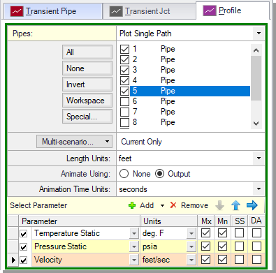
Figure 10: Graph Parameters for Combustion Basket #1 Profile
Note: You can make similar graphs for combustion basket #2. To do so, change the pipe used in the temperature vs time graph to pipe 8, and change the pipes in the animated profile graph to 1, 2, 3, 6, 7, and 8. This would generate similar graphs to the ones seen in and Figure 10.
Step 9. Run the other scenarios and graph the results
Using the Scenario Manager, load the other two scenarios and run them.
Create the same graphs you created for Step
The numerical maximum temperature can be found in the Output window of each scenario and is summarized in Table 1. For these cases the maximum temperatures differ by
Conclusion
Additionally, this example identifies the Estimated Maximum Temperature During Transient as a critical variable in the tabulation of the transient results. This value sets the boundary for the characteristic grid the Method of Characteristics uses. If sonic choking occurs at a temperature higher than the estimated maximum, the model may not converge. As such, this value should be conservatively high on early runs of a model and then refined once the temperature that the transient approaches is known.