Transient Heat Transfer in Pipes

AFT xStream uses a thermal resistance network to account for convective and conductive heat transfer and calculate the steady state heat rates. xStream then uses a discrete solution method to account for radial and axial heat transfer through the pipes and fluid during the transient. This topic discusses the solution methods used by xStream to determine the heat rate and temperatures during the transient. See the Steady State Heat Transfer in Pipes page for information on how the heat rate is derived, and how the convection coefficients are calculated.

Transient Heat Rate

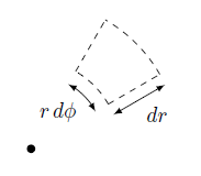
Consider a cylindrical control volume as shown below in Figure 1. Note that dz is perpendicular to the page and thus is not shown.

The heat energy in the control volume due to a change in temperature can be written as:

(1)

The heat energy can also change in response to heat flux and generation:

(2)

By simplifying the heat flux balance and equating it to the heat energy due to temperature change the following is found:

(3)

From Fourier's law for conduction the heat rate is defined as

(4)

By substituting Fourier's law into equation 3 above and dividing the whole equation through by dr dФ dz, the following heat diffusion equation is derived for the radial dimension.

(5)

Transient Pipe Temperatures

xStream will account for heat transfer in the radial and axial directions. However radial heat transfer is dominant, so the below discussion will focus on calculating radial heat transfer.

To calculate the heat rate and temperature profile across the pipe walls and insulation the heat diffusion equation (Equation 5) must be solved. There is not a simple analytical solution for the heat diffusion equation derived above, so a discrete solution method will be used.

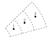
The pipes and insulation layers will each be sectioned radially similar to the example in Figure 2 below, with points 1, 2, and 3 representing calculation nodes at which the temperature and heat rate will be explicitly calculated. Each node represents the temperature, density, and thermal conductivity of the control volume they are within.

There are a few assumptions that are made to calculate the heat rate and temperature.

First, for the purpose of calculating a heat rate xStream assumes a linear temperature profile between each set of consecutive temperature nodes. In reality the temperature would vary logarithmically through a single material. However, using a logarithmic temperature function would be computationally difficult, and provide a negligible increase in accuracy.

Second, the temperature is assumed to be constant at the boundary of different materials, such as where the insulation touches the pipe wall. In reality there would be some contact resistance creating a difference in temperatures between the pipe and insulation, but this is typically a negligible effect.

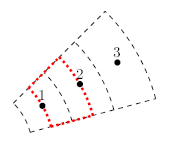
Lastly, for calculation nodes that exist at a boundary between pipe materials, the thermal conductivity and density are assumed to be an average (by volume) of the staggered control volume (Figure 3). This assumption is made to simplify the solution by creating a continuous temperature profile. From testing this assumption provides reasonable results.

Note: The discrete solution method used for calculating radial conduction can potentially become unstable and give physically unrealistic results if the number of radial calculation nodes is insufficient. The default number of nodes should be sufficient for most cases. The number of thermal nodes can be changed on the Sectioning Panel.