Beginner - Tank Blowdown Example (Metric Units)
For the US units version of this example, click here.
This
Topics Covered
-
Model building basics
-
Entering Pipe and Junction data
-
Entering transient data
-
Using the Primary Windows: Workspace, Model Data, Output, & Graph Results
-
Analysis Setup: fluid libraries, sectioning pipes, etc
-
Graph types
-
Workspace Layers
Required Knowledge
This example assumes the user has not used AFT xStream previously. It begins with the most basic elements of laying out the pipes and junctions and solving the transient system via the Method of Characteristics (MOC).
Model File
This example is intended to be built from scratch to help familiarize yourself with the steps to define a complete model in AFT xStream. For reference purposes only, the completed example model file can be found in the Examples folder as part of the AFT xStream installation:
C:\AFT Products\AFT xStream 3\Examples
Step 1. Start AFT xStream
-
ØTo start AFT xStream, open the all applications list in the Windows Start Menu, expand the AFT xStream 3 folder, and choose AFT xStream 3. This refers to the standard menu items created by a standard installation; you may have chosen to specify a different installation location.
As AFT xStream starts, the Startup Window appears, as shown in Figure 1. This window provides you with several options before you start building a model.
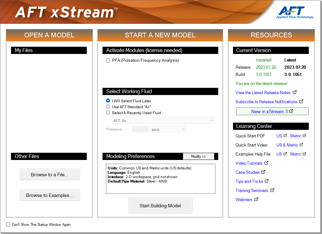
Some of the actions available from the Startup window are:
-
Open a previous model, browse to a model, or browse to an example
-
Activate an Add-on Module
-
Select AFT Standard “Air” or a recently used fluid to be the Working Fluid
-
Review or modify Modeling Preferences: select a Unit System, filter units, choose a Grid Style, select a Default Pipe Material, and more
-
Access other Resources such as Help Files and Video Tutorials
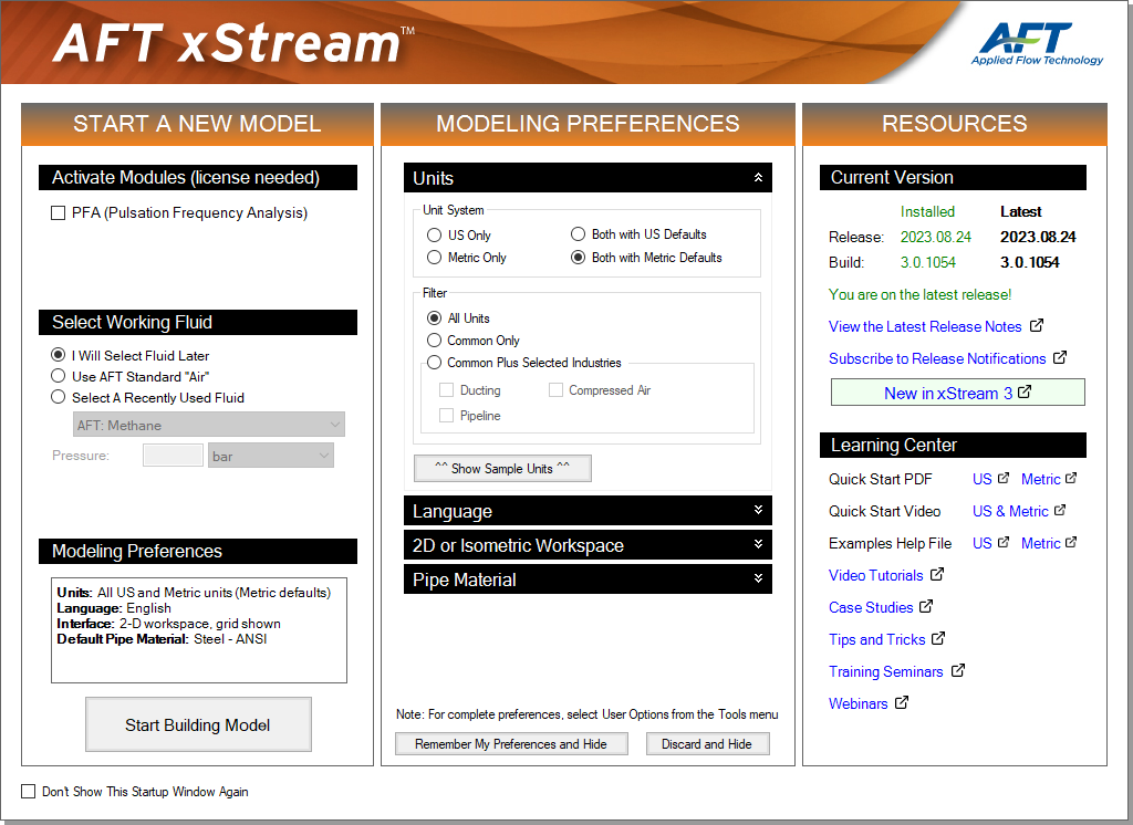
If this is the first time that you have started AFT xStream, Modeling Preferences will be expanded in the middle section of the Startup Window, as shown by Figure 2. If this is not the first time that you have started AFT xStream, the Startup Window will appear with Modeling Preferences Collapsed, as shown in Figure 1.
When collapsed, you can view your current Modeling Preferences at the bottom of the Start a New Model section. To further review or adjust your preferences, click the Modify button (Figure 1).
-
ØWith Modeling Preference expanded, as in Figure 2, select Both with
The Common Plus Selected Industries option adds units from the industries you select. You can use the Show Sample Units option to see the model units based on your selections. After modifying your Modeling Preferences, click Remember My Preferences and Hide.
-
ØClick Start Building Model.
The Workspace window is shown initially, as seen in . The tabs in the AFT xStream window represent the Primary Windows. Each Primary Window contains its own toolbar that is displayed directly beneath the Primary Window tabs.
AFT xStream supports multiple monitor usage. You can click and drag any of the Primary Window tabs off of the main xStream window, where you can then move it anywhere you like on your screen, including onto a second monitor in a dual monitor configuration. To add the Primary Window back to the main xStream window bar, simply click the "X" button in the upper-right of the primary window.
To ensure that your results are the same as those presented in this documentation, this example should be run using all default AFT xStream settings, unless you are specifically instructed to do otherwise.
The Workspace window
The Workspace window is the primary interface for building your model. This window has three main areas: the Toolbox, the Quick Access Panel, and the Workspace itself. The Toolbox is the bundle of tools on the far left. The Quick Access Panel is displayed on the far right. It is possible to collapse the Quick Access Panel by clicking on the thumbtack pin in the upper-right of the Quick Access Panel in order to allow for greater Workspace area.
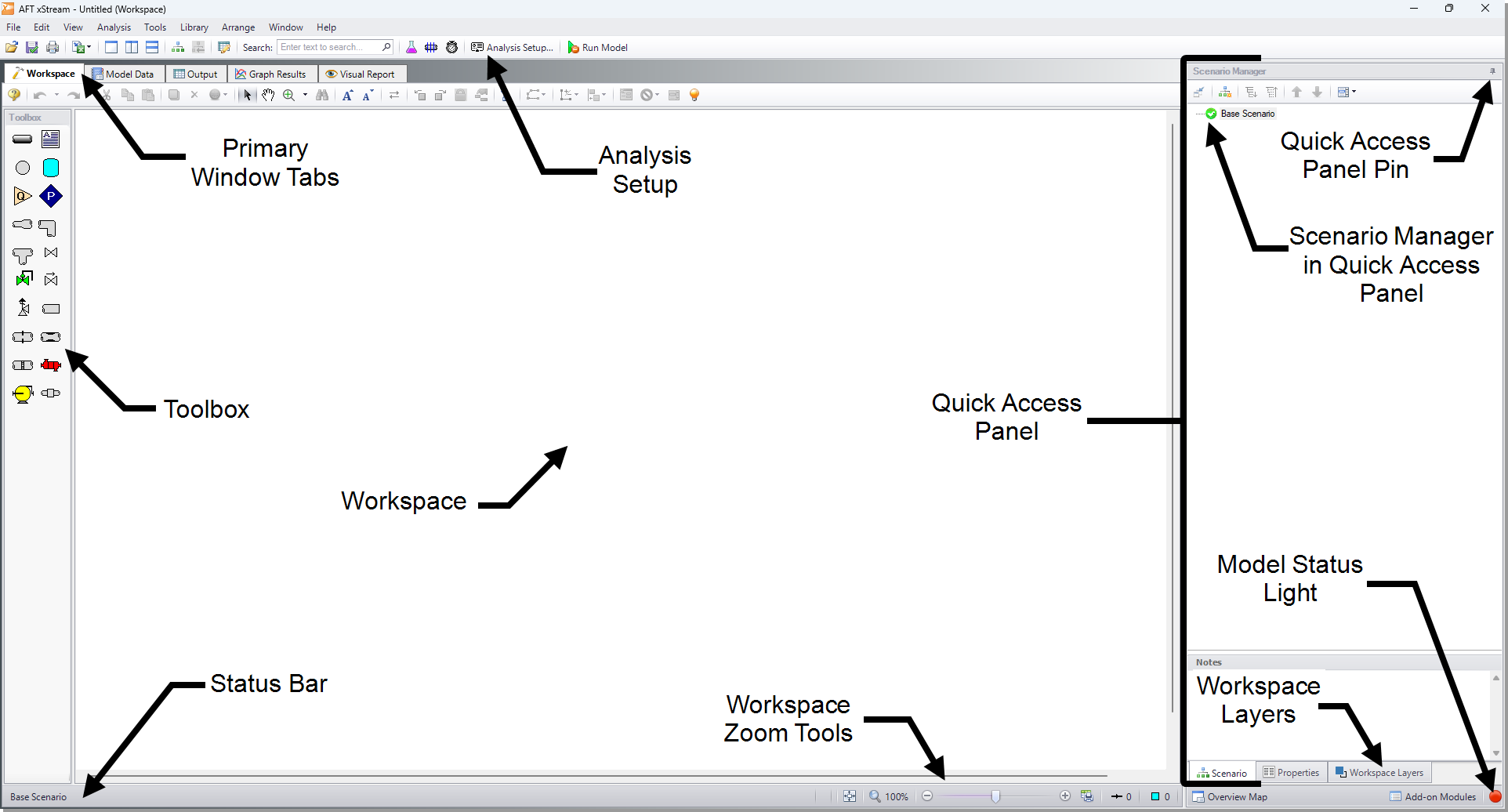
You will build your model on the Workspace using the Toolbox. The Pipe Drawing tool on the upper-left is used to draw new pipes on the Workspace. The Annotation tool beside it allows you to create annotations and auxiliary graphics.
Below the two drawing tools are the different types of junctions available in AFT xStream. Junctions connect pipes and also influence the pressure or flow behavior of the pipe system. Drag and drop any of the junction icons from the Toolbox to add them to the Workspace.
Holding your mouse pointer over a Toolbox icon identifies the tool’s function.
Step 2. Build the model
To lay out this example model, you will place several junctions on the Workspace. Then, you will connect the junctions with pipes.
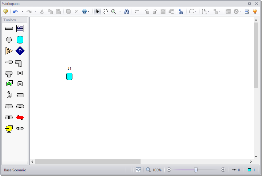
I. Place the Tank junction
-
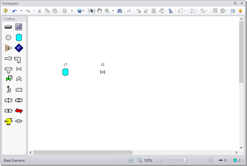
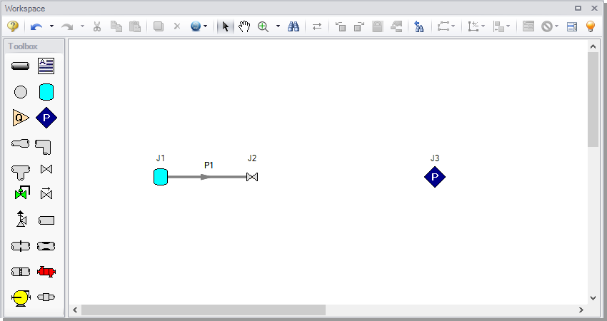
ØTo start, click and drag a Tank junction from the Toolbox and drop it on the Workspace. Figure 4 shows the Workspace with one Tank.
Items placed on the Workspace are called objects. All objects are derived directly or indirectly from the Toolbox. AFT xStream uses three types of objects: pipes, junctions, and annotations.
All pipe and junction objects on the Workspace have an associated ID number. Junctions are prefixed with the letter J, and pipes are prefixed with the letter P. You can assign a name in the object’s Properties window, and the visibility of both the name and ID number can be controlled through the use of Workspace Layers. You can also drag the ID number/name text to a different location to improve visibility.
The Tank you have created on the Workspace will take on the default ID number of 1. You can change this to any desired integer between 1 and 99,999 that is not already assigned.
Editing on the Workspace
You can move junctions on the Workspace to new locations. You can also cut, copy, paste, and duplicate junctions from the Edit menu or using keyboard shortcuts. Undo is available for most arrangement actions on the Workspace.
Note: The relative location of objects is not important. Pipe lengths and junction elevations are defined through property windows. The relative object locations on the Workspace establish the connectivity of the objects but have no bearing on the actual length or elevation relationships.
II. Place the Valve junction
ØTo add a Valve junction, click and drag a valve from the Toolbox and place it on the Workspace as shown in Figure 5. The Valve will be assigned the default number "J2".
III. Place an Assigned Pressure junction
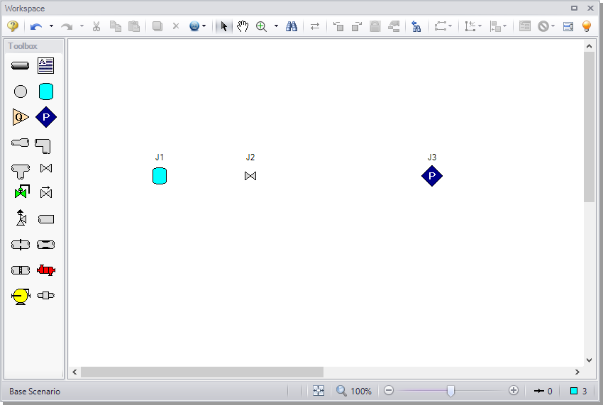
ØTo add an Assigned Pressure junction, click and drag an Assigned Pressure junction from the Toolbox and place it on the Workspace as shown in Figure 6. The Assigned Pressure junction will be assigned the default number "J3".
-
ØBefore continuing, save the work you have done so far by either choosing Save As... from the File menu, clicking the Save button on the Common Toolbar, or using the CTRL+S keyboard shortcut. Enter a file name (Tank Blowdown, perhaps) and AFT xStream will append the *.xtr extension to the file name.
IV. Draw a pipe between J1 and J2
Now that you have all of the junctions placed, you need to connect them with pipes.
-
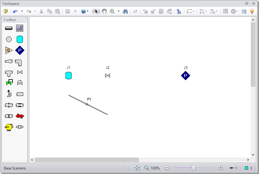
ØTo create a pipe, click the Pipe Drawing Tool icon on the Toolbox. The pointer will change to a crosshair when you move it over the Workspace. Draw a pipe near the junctions by clicking and dragging the mouse, similar to that shown in Figure 7.
The pipe object on the Workspace has an ID number (P1) that is shown near the center of the pipe.
-
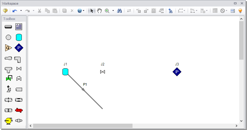
ØTo place the pipe between J1 and J2, use the mouse to grab the pipe in the center and drag it so that the left endpoint falls within the J1 Tank icon, then drop it there (see Figure 8). Next, grab the right endpoint of the pipe and stretch the pipe, dragging it until the endpoint terminates within the J2 Valve icon (see Figure 9).
V. Add the remaining pipe
A faster way to add a pipe is to draw it directly between the desired junctions.
-
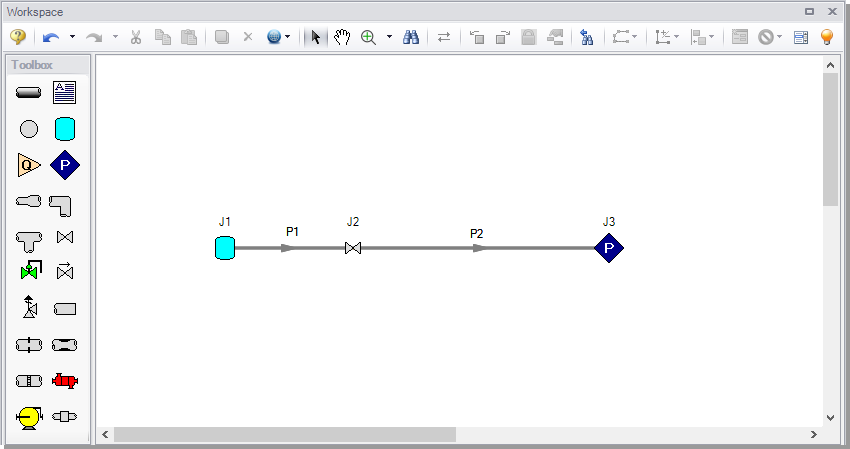
ØActivate the Pipe Drawing Tool again. Position the cursor on the J2 Valve, then press and hold the left mouse button. Stretch the pipe across to the J3 Assigned Pressure junction, then release the mouse button. All objects in the model should now be graphically connected as they are in Figure 10.
Save the model by selecting "Save" in the File menu, by clicking the "Save" icon on the Toolbar, or by entering CTRL+S.
Reference positive flow direction
The arrow on each pipe indicates the reference positive flow direction for the pipe. The direction does not influence the direction that the flow may go, it influences sign convention only. If the direction of flow calculated by the Solver is the opposite of this reference flow direction, then the output will show the flow rate as a negative number.
You can reverse the reference positive flow direction by choosing Reverse Direction from the Arrange menu, selecting the Reverse Pipe Direction button on the Toolbar, or pressing F3.
Although the reference positive flow direction does not need to point in the direction of the actual flow, when used with compressors, the reference direction determines the suction side and discharge side of the compressor.
Note: Examples of other junctions that depend on pipe directions include Control Valves, Check Valves, and Area Changes.
Note: Some users find it desirable to lock objects to the Workspace once placed. This prevents accidental movement and disruption of the connections. You can lock all the objects by first selecting all objects by using CTRL+A or the Edit menu by clicking Select All. Then use CTRL+L or go to the Arrange menu and selecting Lock Object. The lock button on the Workspace Toolbar will appear depressed, indicating it is in an enabled state. Alternatively, you can use the grid feature and snap to grid. The grid options can be modified through the Arrange menu or User Options window.
A. Define the model components
The model must have all pipes and junctions defined in order for it to run. This step encompasses the proper input data and connectivity for all pipes and junctions.
Object status
Each pipe and junction has an object status. The object status tells you whether the object is defined according to AFT xStream's requirements. To see the status of the objects in your model, click the light bulb icon on the Workspace Toolbar (alternatively, you could choose Show Object Status from the View menu). Each time you click the light bulb, Show Object Status is toggled on or off.
When Show Object Status is on, the ID numbers for all undefined pipes and junctions are displayed in red on the Workspace. Objects that are completely defined have their ID numbers displayed in black. These colors are configurable through User Options from the Tools menu.
Because you have not yet defined the pipes and junctions in this model, all the object ID numbers will change to red when you turn on Show Object Status.
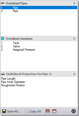
Another useful feature is the List Undefined Objects window (Figure 11). This can be opened from the View menu by clicking on List Undefined Objects, or by clicking the List Undefined Objects icon on the Workspace toolbar . All objects with incomplete information are listed. Click on an undefined pipe or junction to display the property data that is missing. Click the close button on the bottom-right to stop showing this window.
I. Enter data for the J1 Tank
-
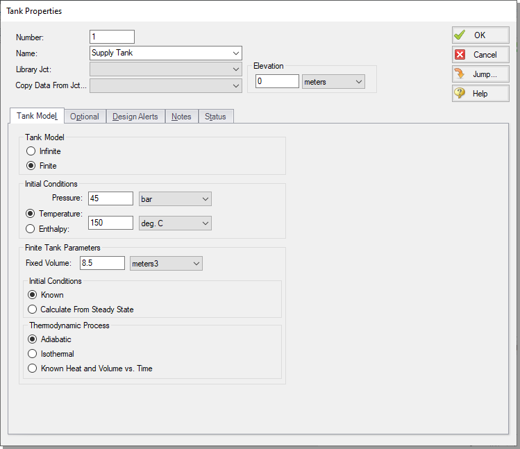
ØTo define the first tank, open the J1 Tank Properties window (Figure 12) by double-clicking on the J1 junction.
Note: You can also open an object’s Properties window by selecting the object (clicking on it) and then either pressing the Enter key or clicking the Open Pipe/Junction Window icon on the Workspace Toolbar.
-
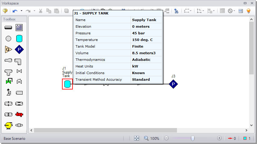
ØEnter the following properties into the J1 Tank Properties window:
-
Name = Supply Tank
-
Elevation = 0
-
Tank Model = Finite
-
Pressure =
-
Temperature =
-
Fixed Volume =
-
Initial Conditions = Known
-
Thermodynamic Process = Adiabatic
-
Note: You can specify default units for many parameters (such as
You can give the junction a name, if desired, by entering it in the Name field at the top of the window. By default, the junction's name indicates the junction type, and will be displayed in the Model Data and Output. It can optionally be displayed on the Workspace via the use of Workspace Layers which will be discussed later.
Most junction types can be entered into a custom Junction Library allowing the junction to be used multiple times or shared between users. To select a junction from the custom library, choose the desired junction from the Library List in the junction's Properties window. The current junction will get the properties from the library component.
The Copy Data From Jct... list will show all the junctions of the same type in the model. This will copy desired parameters from an existing junction in the model to the current junction.
Using the tabs in the Properties windows
The information in the Properties windows is grouped into several categories and placed on separate tabs. Click the tab to bring its information forward. Figure 12 is an example of a Tank’s Properties window.
The Tank Model tab is the tab that appears first when the Tank junction is opened and contains all of the inputs required to define the Tank in steady-state. While the Tank Model tab is specific to the Tank junction, the first tab opened for any junction will contain all inputs required for that junction to be defined.
The Optional tab allows you to set Special Conditions (like closing a valve or turning off a compressor), and change the junction icon.
Each junction has a tab for Notes, allowing you to enter text describing the junction or documenting any assumptions.
The highlight feature (on by default) displays all the required information in the Properties window in light blue. You can toggle the highlight on and off by pressing F2 with the properties window open or by double-clicking an empty area above the tabs of the properties window. The highlight feature can also be turned on or off by selecting Highlight in Pipe and Jct Windows from the View menu.
The Status tab will state whether all required input data is present for a given junction. If not, it will list all inputs that are incomplete.
-
ØClick OK. If Show Object Status is turned on, you should see the J1 ID number turn black again, telling you that J1 is now completely defined.
You can check the input parameters for J1 quickly, in read-only fashion, by using the Inspection feature. Position the cursor on the Tank J1 junction and hold down the right mouse button. An information box appears, as shown in Figure 13.
Inspecting is a faster way of examining the input (and output if results are available) than opening the Properties window.
II. Enter data for the J2 Valve
The Valve is the element which will cause the transient in this model. The purpose of the model will be to understand how the conditions within the supply tank and discharge pipe change after the valve opens.
-
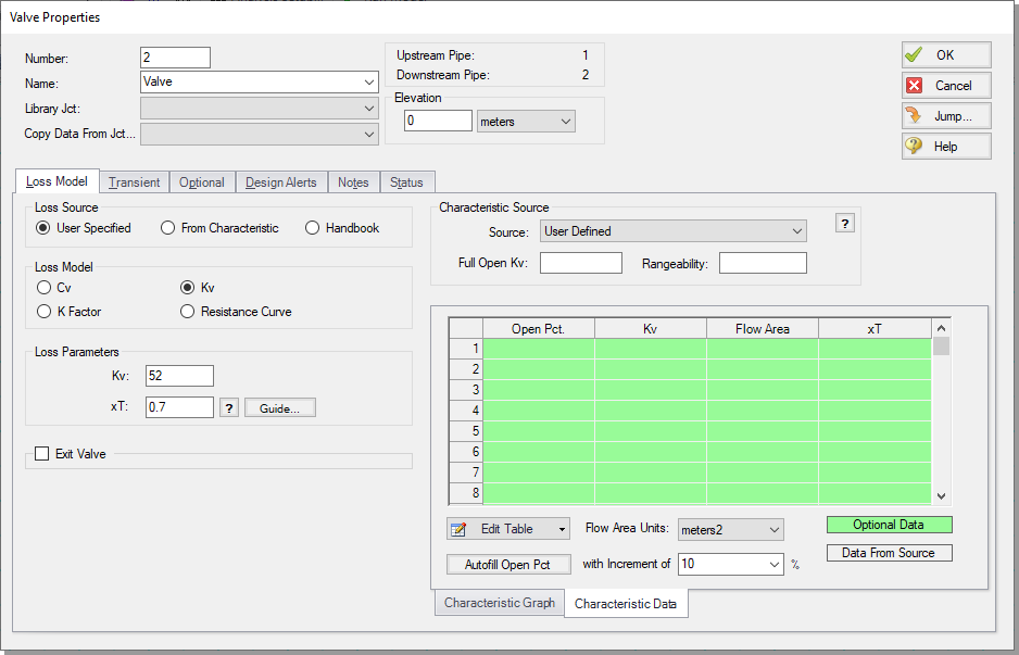
ØDouble-click the J2 junction icon to open the Valve Properties window and enter the following data on the Loss Model tab (Figure 14).
-
Elevation = 0
-
Loss Source = User Specified
-
Loss Model =
-
-
xT = 0.7
-
-
ØClick the Optional tab and set the Special Condition to Closed. This will set the initial steady-state
-
ØClick the Transient tab and enter the following data (Figure 15).
-
Initiation of Transient = Time (indicates that the valve closure will be initiated at the time you specify)
-
Enter the following
Time (seconds) Kv xT 0 0 0.7 0.1 52 0.7 240 52 0.7
The first data point of the table must match the steady-state value of the junction; therefore, the values are grayed out. In this case, the valve is closed in the initial steady-state due to the Special Condition specified in the previous step. Therefore, the initial transient data point automatically populates the valve as being closed (
-
-
ØClick the OK button to save and close the Valve Properties window. There should now be a “T” symbol next to the Valve junction on the Workspace, indicating that transient data is entered for the junction. The Valve junction on the Workspace will additionally have a red “X” next to it indicating that the junction contains a Special Condition.
III. Enter data for the J3 Assigned Pressure
-
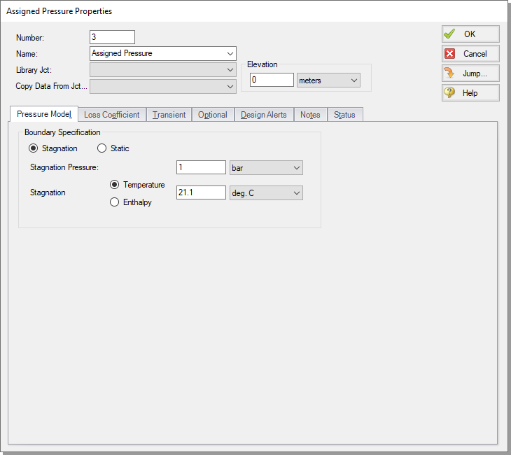
ØDouble-click the J3 junction icon to open the Assigned Pressure Properties window and enter the following data (Figure 16).
-
Elevation = 0
-
Boundary Specification = Stagnation
-
Stagnation Pressure =
-
Temperature =
-
Click the OK button to save and close the Assigned Pressure Properties window
ØSave the model again before proceeding.
IV. Enter data for Pipe P1
Data for pipes and junctions can be entered in any order. In this example, the junctions were done first. The next step is to define all of the pipes.
-
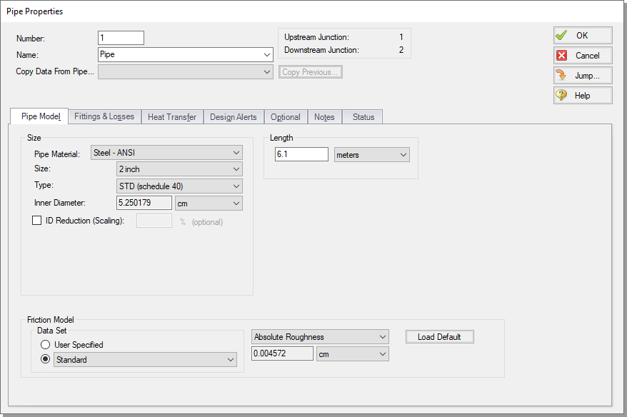
ØOpen the Pipe Properties window for Pipe P1. The Pipe Model tab opens by default (Figure 17).
-
Pipe Material = Steel - ANSI
-
Size = 2 inch
-
Type = STD (schedule 40)
-
Length =
-
Friction Model = Standard
The Inspect feature can be accessed not only from pipes and junctions located on the Workspace, but also from within the Properties window of each pipe (and certain junctions). This is helpful when you want to quickly check the properties of objects that connect to a pipe or junction whose Properties window you already have open.
To Inspect a junction connected to a given pipe, position the mouse pointer on the connected junction’s ID number in that pipe’s Properties window (located at the top right of the Pipe Properties window) and hold down the right mouse button. This process can be repeated for any junction that states the upstream and downstream pipe in the junction’s Properties window. You can jump to that junction’s Properties window by double-clicking the connected junction’s ID number, or use the Jump button to jump to any other part of the model.
-
ØClick OK to save and close the Pipe Properties window for Pipe P1.
V. Enter data for Pipe P2
-
ØOpen the Pipe Properties window for Pipe P2 and enter the following data:
-
Pipe Material = Steel - ANSI
-
Size = 2 inch
-
Type = STD (schedule 40)
-
Length =
-
Friction Model = Standard
-
Click OK to save and close the Pipe P2 Properties window.
-
ØCheck if all the pipes and junctions are defined by clicking on the List Undefined Objects button. If all data is entered, no items should appear in the Undefined Objects window. If items are present, open the corresponding Properties windows for the incomplete items from the Workspace. The Status tab on each Properties window will indicate what information is missing.
B. Review model data
-
ØSave the model. It is also a good idea to review the input using the Model Data window.
Reviewing input in the Model Data window
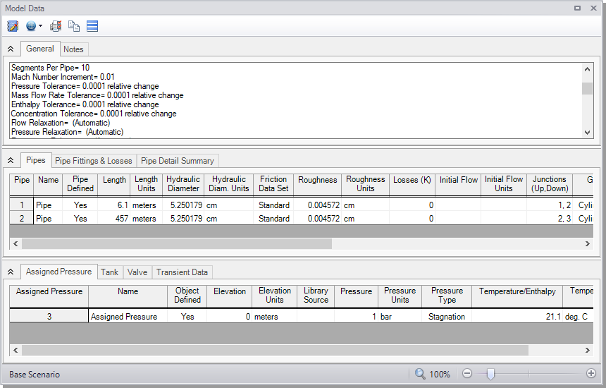
The Model Data window is shown in Figure 18. To change to this window, you can click on the Model Data tab, select it from the Window menu, or use the CTRL+M keyboard shortcut. The Model Data window gives you a table-based perspective of your model. Selections can be copied to the clipboard and transferred into other Windows programs, saved to a formatted file, printed to a PDF, or printed out for review. Figure 19 shows an expanded view of the Transient Data tab from Figure 18. Here, all transient input data for the model is shown.
Data is displayed in three general areas. The top is called the General data section, the middle is the Pipe data section and the bottom is the Junction data section. Each section is collapsible using the button at the top-left of the section. Further, each section can be resized.
The Model Data window allows access to all Properties windows by double-clicking on any input parameter column in the row of the pipe or junction you want to access.
Step 3. Specify Analysis Setup
The Analysis Setup window allows the user to define fluid properties, view undefined pipe/junction properties, section pipes, adjust simulation duration, enable Add-on Modules if purchased and available on the current license, and specify other simulation settings from a single central location.
-
ØClick Analysis Setup on the Main Toolbar to open the Analysis Setup window (see Figure 20). The Analysis Setup window contains various groups depending on which modules you may be using. Each group has one or more items. A fully defined group has every item within it defined with all required inputs. Complete every group to run the Solver. A group or item that needs more information will have a red exclamation mark to the left of the group or item name. After completing a group, the group icon shows a green circle with a checkmark. After defining all groups, thus completing the Analysis Setup, the Model Status light in the lower-right corner of the Workspace turns from red to green.
The Analysis Setup window can also be opened by clicking on the Model Status Light on the Status Bar at the bottom-right corner of the AFT xStream window (Figure 3).
A. Modules
Under the Modules group, click on the Modules item to open the Modules panel, shown in Figure 20. Here you can enable and disable the Pulsation Frequency Analysis (PFA) Add-on Module if it is available on the license. By default, the model will have all modules disabled. Make no changes to this panel for this example.
-
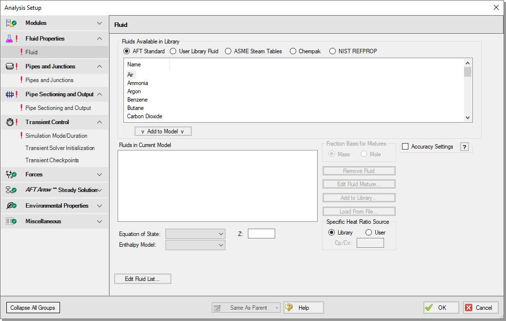
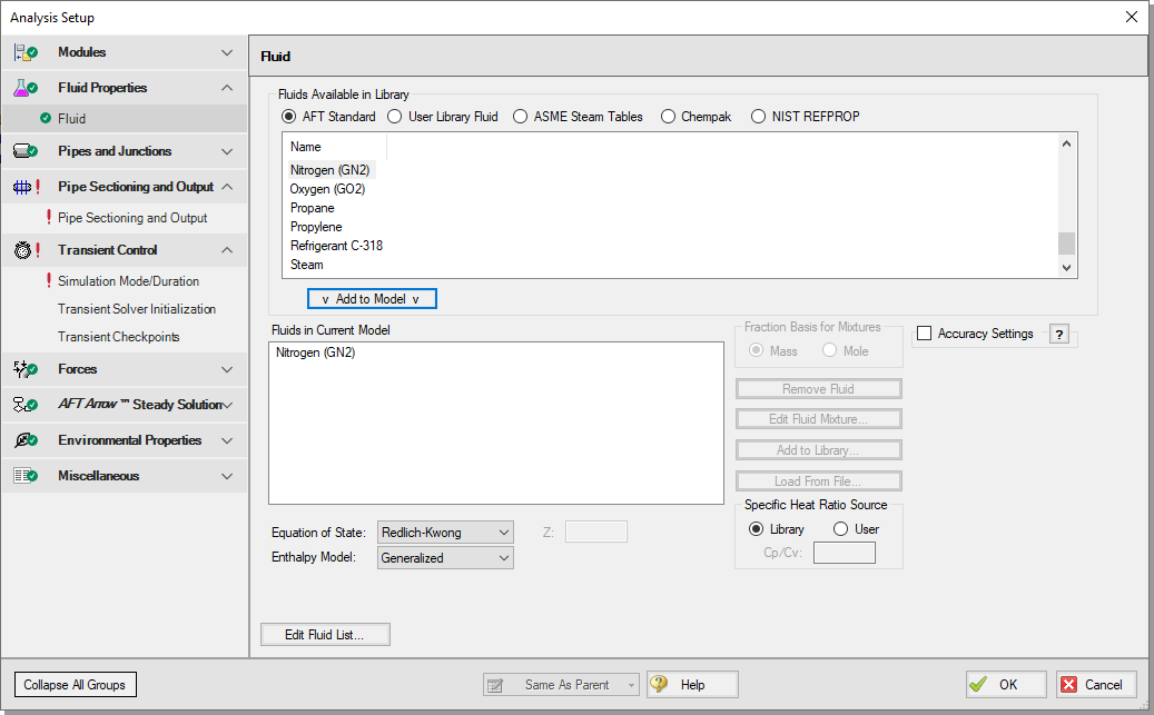
ØSelect the Fluid item to open the Fluid panel (Figure 21).
This panel allows you to specify the fluid used in the model. There are several fluid libraries that are available:
-
AFT Standard - Common fluids from various industry standard sources have been curve fit to optimize calculation speed.
-
User Library Fluid - If the desired working fluid is not available via the other sources, custom fluid properties can be entered and saved to the User Library for repeated use in the future. Custom fluids are created by opening the Library Manager from the Library menu or by clicking the Edit Fluid List button in the Fluid panel and clicking Add New Fluid.
-
ASME Steam Tables - Properties are calculated via the Equations of State which were used to generate the classic steam/water tables in the IAPWS Industrial Formulation (1997).
-
Chempak - Optional add-on for purchase which contains data for several hundred fluids and supports user-specified fluid mixtures. Chempak is licensed from Madison Technical Software.
-
NIST REFPROP - The Reference Fluid Thermodynamic and Transport Properties (REFPROP) Database is licensed from the National Institute of Standards and Technology (NIST) where properties for approximately 150 fluids are calculated via Equations of State. REFPROP supports user-specified fluid mixtures.
-
ØSelect the AFT Standard fluid option, then choose Nitrogen (GN2) from the list and click the Add to Model button. Leave the Equation of State as Redlich-Kwong and the Enthalpy Model as Generalized.
C. Pipes and Junctions
The Pipes and Junctions panel is used to show the status of the pipes and junctions on the Workspace. This item is incomplete if there are any undefined pipes/junctions on the Workspace, or if there are no pipes/junctions on the Workspace. In this example the objects in the Workspace are fully defined, so this item is marked as complete.
Running models in steady-state
After fully specifying the Fluid panel and the pipes and junctions, sufficient information exists to run the model in steady-state. You can run the model in steady-state by selecting the Simulation Mode/Duration panel from the Transient Control group and then choosing AFT Arrow™ Steady for the Time Simulation. If you do this, the other inputs on the Simulation Mode/Duration panel and the Pipe Sectioning and Output panel will no longer be required, and the model can be run.
In general, it is a good idea to always run your model in steady-state before running the full transient analysis to make sure the model is giving reasonable results. However, in this case the model has no flow in the steady-state due to the closed valve, and a steady-state run is trivial. Keep the Transient option selected.
D. Pipe Sectioning and Output
The next panel is the Pipe Sectioning and Output panel in the corresponding group. The Pipe Sectioning and Output panel divides pipes into computation sections in a manner which is consistent with the Method of Characteristics (MOC).
To satisfy the MOC, the following equation must be valid:

where Δt is the time step, Δx is the section length, and c is the sonic velocity.
-
ØEnter 1 for the Minimum Number of Sections Per Pipe.
The Minimum Number of Sections Per Pipe determines the section length by taking the quotient of the shortest pipe's length and the Minimum Number of Sections. Increasing the number of sections in a model will always have a positive correlation to the model accuracy as the error inherent to the Method of Characteristics decreases when the step size is made smaller. However, the run time of the model increases quadratically as well, since each added section to the shortest pipe increases the number of calculations for each time step. This increase in run time is exacerbated when there is a large disparity between the minimum pipe length and the length of the longest pipe, such as the case in this model.
The Minimum Number of Sections Per Pipe for this example will be set to 1 for expediency, but note that it would be wise to use more computational sections if you are running an AFT xStream model for real projects. Typically, less sections and faster run time is useful during the initial model development and troubleshooting, and more sections can be used for final runs.
-
ØDefine the Estimated Maximum Pipe Temperature During Transient as
The Estimated Maximum Pipe Temperature During Transient is used to calculate the maximum sonic velocity. Since all pipes in the network must be solved together, the time step must be the same for each pipe. However, the sonic velocity will not be equivalent for all of the pipes. Therefore, the sonic velocity at the specified maximum temperature is used to find a uniform time step for the system. Without a uniform time step, the MOC could fail. Choosing a maximum temperature that is much higher or much lower than the maximum temperature calculated during the run can result in additional uncertainty in the MOC solution
The Estimated Maximum Pipe Mach Number During Transient is an additional parameter that affects result accuracy. The value of this parameter is set to 1 by default so that the Method of Characteristics grid is able to bound the sonic velocity obtained at the Estimated Maximum Pipe Temperature During Transient. Setting the Mach number to 1 ensures that the model will not fail assuming the input values for that variable are correct.
However, because of the computational methodology of the MOC, using the default Mach number can introduce error due to the difference between the Estimated Maximum Pipe Mach Number During Transient and the actual maximum. This error is particularly noticeable when the Mach number during the simulation is near zero. If the maximum Mach number reached during the simulation is near zero, a more accurate model can be found by lowering the estimated maximum based on the actual Maximum Mach number of the system.
To change the Estimated Maximum Pipe Mach Number During Transient, you must expand the Advanced Sectioning Controls dropdown in the Pipe Sectioning and Output panel of Analysis Setup. It is highly recommended that you first run the model with the default Mach number in order to ensure that choking does not occur in the pipes before altering this number. Additionally, be cognizant of the fact that altering sectioning, transient components, or maximum estimated temperatures between runs could have an effect on the maximum Mach number reached during the simulation. As such, it is generally recommended to only change this number once your model has reached a more finalized state.
Sonic choking will be seen in this model, so no adjustment to Maximum Mach Number will be made.
The Sectioning Summary underneath the inputs will be partially filled in. Certain properties such as the Estimated Total Steps and Total Pipe Computations will need the Simulation Mode/Duration panel to be completed before values can be displayed.
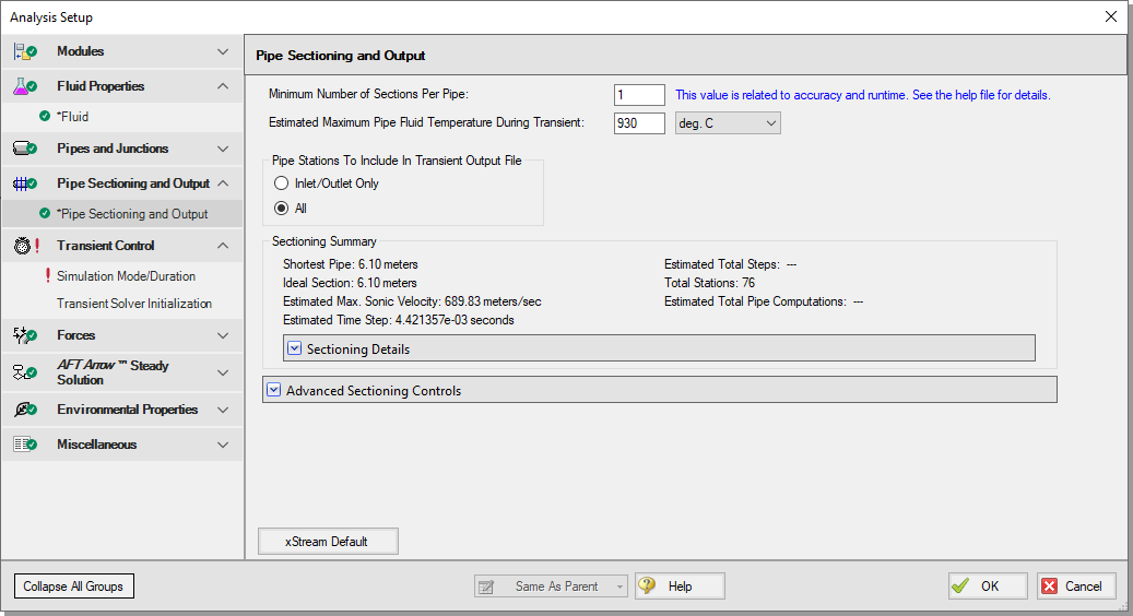
Figure 22: The Sectioning panel in the Analysis Setup window is used to calculate the time step of the model
-
ØSelect the Simulation Mode/Duration panel. Enter 0 seconds for the Start Time and 240 seconds for the Stop Time (Figure 23).
-
ØClick OK to accept the changes in Analysis Setup.
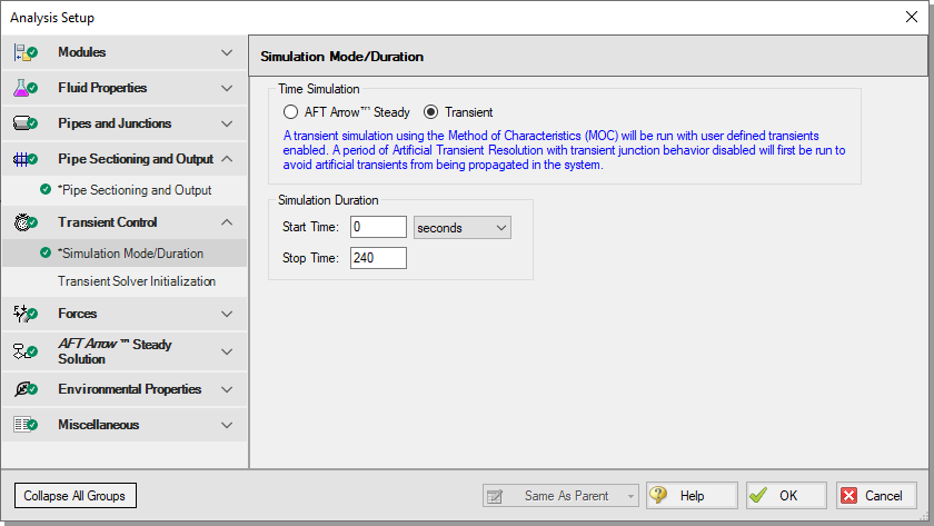
Figure 23: The Simulation Mode/Duration panel is used to specify the simulation type and the time span for the transient
-
ØSave the model.
Step 4. Run the model
-
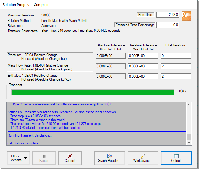
ØChoose Run Model... from the Analysis menu or click the Run Model button on the Common Toolbar. During execution, the Solution Progress window is displayed and can be used to pause or cancel the Solver's activity (Figure 24).
This simple model will take several minutes to run. A typical xStream model may take hours to solve depending on the simulation duration, sectioning, and which fluid library is used.
The two Solvers
AFT xStream has two Solvers. The first is called the AFT Arrow™ Steady Solver, which as its name suggests, obtains a steady-state solution to the pipe network. The second Solver is called the Transient Solver and solves the gas transient equations via the Method of Characteristics (MOC).
The AFT Arrow™ Steady Solver and Transient Solver use different sectioning methods which causes small discrepancies between the converged AFT Arrow™ Steady solution and the first time step of the transient solution. AFT xStream runs the Transient Solver for a period of time before the transient simulation begins in order to allow these artificial waves caused by these discrepancies to dampen and die out. Once the artificial transients have settled, AFT xStream checks the solution with resolved artificial transients against the AFT Arrow™ Steady solution. If the mismatch between the beginning and end of the artificial transient resolution process is sufficiently small AFT xStream proceeds with the transient simulation. See the chart in Figure 25 as a visual representation of the process described above.
![]()
Figure 25: Illustration of the Transient Solver Initialization process with artificial transient resolution
-
ØWhen the solution is obtained, click the Output button to display the table-based Output window. The information in the Output window can be reviewed visually on the screen, saved to a file, exported to a spreadsheet-ready format, copied to the clipboard, or printed.
When the Solver runs, the output data is written to a file. This file is given the same name as the model itself with a number appended to the name, and with an *.out extension appended to the end. For all data processing, graphing, etc., the data is extracted from this file. The number is appended because users are able to build different scenarios all within this model. Each scenario will have its own output file; thus, the files need to be distinguishable from each other.
The output file will only remain on disk if you save the model after it has been run. Once saved, it will remain until the user erases it or the model input data is modified.
-
ØSave the model file again such that the output file is saved to the disk. This means that if you were to close your model right now and then reopen it, you could proceed directly to the Output window for data review without rerunning your model.
Step 5. Review the Output window
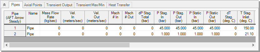
The Output window (Figure 26) is similar in structure to the Model Data window. Three areas are shown, and you can minimize or enlarge each section by clicking the arrow next to the General, Pipes, and All Junctions tabs. The items displayed in the tabs can be customized with the Output Control window, which can be opened by clicking the spreadsheet with a pencil icon from the Common Toolbar or from the Tools dropdown menu.
The General section will open by default to the Warnings tab if any Warnings or Cautions were encountered during the simulation. This model should generate a Caution that the Maximum Transient Pipe Mach Number is at least 0.2 higher than the steady pipe Mach number, which occurs since there is no flow in the system at steady-state. When this Caution is present, the effect of pipe sectioning on results can be significant. The impact of pipe sectioning will be addressed in greater detail in a later step.
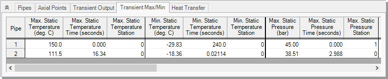
The Output window allows you to review both the steady-state and transient results. The Pipes tab, All Junctions tab, and any specific junction tabs in the Junction section (such as Tank, Valve, etc.) show the steady-state results. A summary of the maximum and minimum transient results for each pipe is given on the Transient Max/Min tab in the Pipe section and is the active tab displayed in Figure 26. You can review the solutions for each time step (i.e., a time history) on the Transient Output tab shown in Figure 27. Note that in order to display all pipe stations the model will need to be set to save data for all stations. By default, xStream saves all data points. This can be changed in the Pipe Sectioning and Output panel.
-
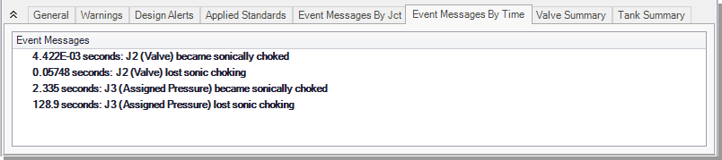
ØClick on the Event Messages By Time tab. This tab allows you to review changes of states at junctions, such as the onset of choking or the initiation of transient events (see Figure 29). There should be messages indicating that the J2 Valve experienced a near instantaneous choking that dissipated after about 0.06 seconds while the J3 Assigned Pressure experienced choking after 2.
The Output Control window (Figure 30) can be accessed from either the Tools menu or from the Output window Toolbar, and it allows you to select the specific output parameters you want to display in the Output window. You can choose the units and reorder the parameters as desired. If you do not change any of the Output Control settings, the default Output Control parameters are assigned.
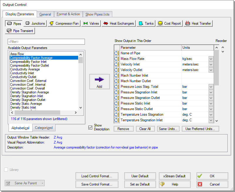
Units for each column in the Output window can also be changed by double-clicking the column header. This will open a window in which you can select the units you prefer (Figure 31). These changes are extended to the Output Control parameter data that is set.
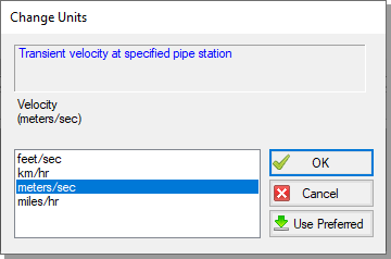
Figure 31: The Change Units window is opened from the Output window tabs by double-clicking a column header
Step 6. View the Graph Results
For transient analysis, the Graph Results window will usually be more helpful than the Output window because of the more voluminous data.
-
ØOpen the Graph Results window by clicking the Graph Results tab, choosing it from the Windows menu, or by pressing CTRL+G.
Figure 32 shows the Graph Results window with the Graph Control tab selected on the Quick Access Panel.
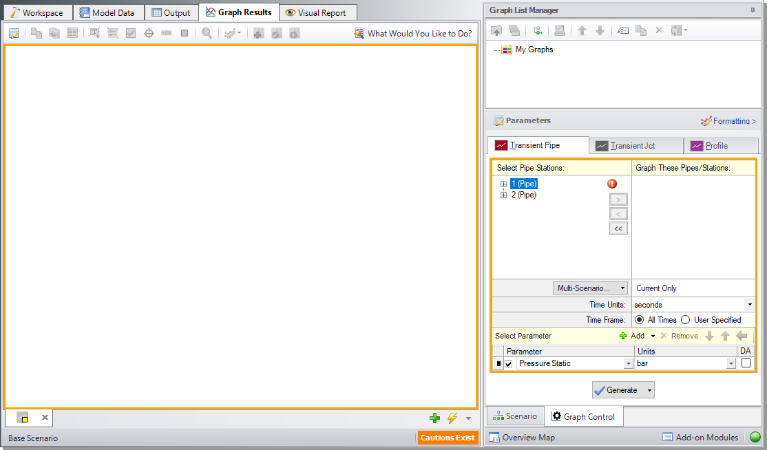
Figure 32: The Graph Results window and Quick Access Panel Graph Control tab is where various system parameters (both steady-state and transient) can be graphed
A. Create a Transient Pipe graph
AFT xStream gives you the ability to create stacked graphs. These are graphs that are vertically aligned such that they use the same same x-axis but have different parameters on the y-axis of each graph. This feature is helpful when you want to look at how different parameters vary with time at a given position without having to create separate graphs.
-
ØAccess the graphing parameters by opening the Graph Control tab on the Quick Access Panel (this tab is automatically selected when the Graph Results window is opened). Because we are interested in seeing how the pressures and flows in specific pipe sections respond over time, ensure that the Transient Pipe tab is selected in the Parameters/Formatting area on the Quick Access Panel. Alternatively, you can open the Select Graph Parameters window by clicking on the corresponding icon on the Graph Results Toolbar (Figure 32).
-
ØAdd the Pipe P2 Outlet to the Graph These Pipes/Stations list by expanding the tree for Pipe P2 under the Select Pipe Stations list and double-clicking the Outlet station. Pipe P2 Outlet represents the pipe computing station at the discharge of the blowdown pipe. Alternatively, you can click on the right arrow button after selecting the pipe station you want to graph to add it to the Graph These Pipes/Stations list.
-
ØVerify the Time Units are set to seconds and the Time Frame is set to All Times.
-
ØClick the Add button twice, which is the green “+” icon next to Select Parameter. Two new rows will appear under the Parameter definition area which will create stacked graphs (Figure 33).
-
ØSelect the following parameters from the dropdown lists on each row:
-
Temperature Static with units of deg.
-
Velocity with units of
-
Mach Number
-
Figure 33 shows the input in the Parameters/Formatting area on the Quick Access Panel.
![]()
Figure 33: The Graph Control tab on the Quick Access Panel allows you to specify the graph parameters you want to graph in the Parameters/Formatting area
-
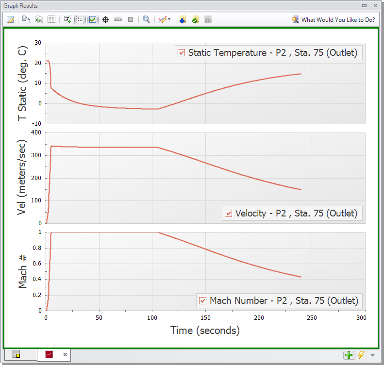
ØClick the Generate button at the bottom of the Quick Access Panel to create the static temperature, velocity, and Mach number graphs at the pipe discharge over the duration of the simulation.
-
ØFormat the legend font size to 20 pt by right-clicking on any legend and using the scroll bar. Drag the legend to the top-right corner of the graph.
-
ØFormat the y-axis and x-axis font size to 20 pt by right-clicking on each axis parameter and using the scroll bar.
Figure 34 shows the stacked graphs detailing the static temperature, velocity, and the Mach number at Pipe P2 outlet over the course of 240 seconds. Here you can see that the maximum temperature at the discharge is about
Note: The axis titles in the stacked graphs in Figure 34 have been modified for clarity.
The Formatting area on the Graph Control tab can be used to modify the graph colors, fonts, and other elements. Options to copy the graph image or x-y data are available on the Graph Results Toolbar or by right-clicking the graph. The graph image or x-y data can be saved from the File menu.
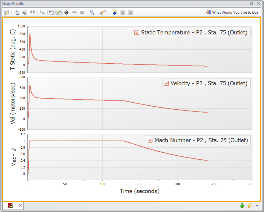
Further review of the graph results in Figure 34 shows that sonic choking occurs after several seconds, as was seen on the Event Messages tab in the Output window, and continues for the next
B. Create a Transient Junction graph
For the purpose of this analysis, it is also helpful to look at the temperature and pressure of the tank over time.
-
ØCreate a new graph tab by clicking the New Tab button which is the green plus icon located on the bottom-right, immediately below the graph area (Figure 32).
-
ØClick the Transient Jct tab on the Graph Control tab of the Quick Access Panel (Figure 35). Add the J1 (Supply Tank) junction.
-
ØVerify the Time Units are set to seconds and the Time Frame is set to All Times.
-
ØClick the Add button to add a new row under the Parameter definition area.
-
ØSelect the following parameters from the dropdown lists on each row:
-
Pressure Stagnation with units of
-
Temperature Stagnation with units of deg.
-
-
ØClick the Generate button. These graphs show the tank pressure and temperature initially decrease quickly, then decrease more slowly as time progresses. This change in slope is due to a decreasing pressure gradient between the tank and the atmosphere as the tank is emptied, which slows the mass flow rate out of the tank (Figure 36).
Note: AFT xStream assumes all pipes are adiabatic (perfectly insulated). Over a 240 second run time this assumption may not be accurate. Consider this when evaluating simulation results over longer times.
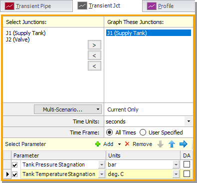
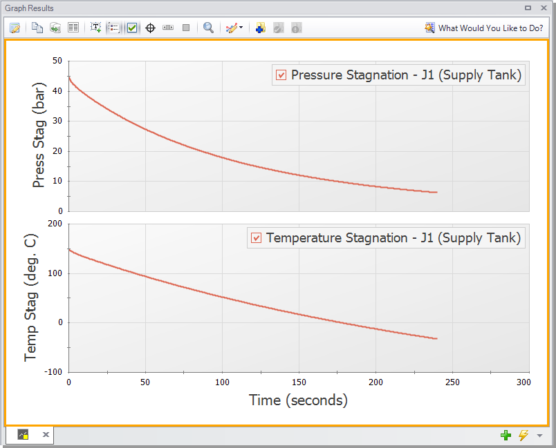
Figure 36: The Transient Junction graph shows how variables within a junction change over time, such as with the temperature and pressure of Tank J1
This junction graph could be used to determine when certain conditions within the tank were met. For instance, suppose there was a need to know when the tank pressure dropped below
C. Create an Animated Profile graph
Lastly, we will animate the profile of the system to show the wave caused by opening the valve.
-
ØCreate a new graph tab and select the Profile tab. Under Plot Single Path, select Pipe P1 and P2. After ensuring your Length Units are
ØAdd new parameters until you have 4 in total, and set them to the following (see Figure 37):
-
Pressure Static with units of
-
Temperature Static with units of deg.
-
Velocity with units of
-
Density Static with units of
-
-
ØClick the Generate button. This will show the max and min envelopes of the parameters throughout the selected time frame. The animation can started by clicking Play in the top-left playback controls (Figure 38).
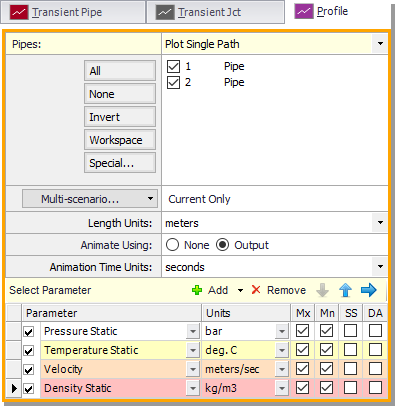
Figure 38: The Profile Graph show the Maximum and Minimum values of all parameters shown in the Graph over the specified time Frame, and can also animate the values
Take note of the pressure wave that is created at the valve just after animation is started. This wave travels to the Assigned Pressure junction before reflecting back towards the valve. The amount of time it takes this wave to travel to the reflection point and back is called the communication time. It should be noted when creating your transient that any event which occurs over a shorter length of time than the communication time of the system is considered to happen instantaneously.
Step 7. View the Workspace Layers
Workspace Layers can display input and output values superimposed over the model, and color pipes automatically based on output values.
The Workspace Layers can also animate the transient pipe results in a color animation overlaid on the model.
-
ØNavigate to the Workspace window by clicking on the Workspace tab or pressing CTRL+W. Select the Workspace Layers tab in the bottom-right of the Quick Access Panel. The Workspace Layers panel contains two sections named Layer Presets and Layers.
Within the Layers section, there are two expandable or collapsible groups which contain the two layer types named Color Maps and Standard layers. We will integrate the model results with the graphical layout of the pipe network by using the All Objects Layer located under the Standard group. The All Objects Layer is the bottommost layer for all models and shows all pipes, junctions, and annotations when the layer is visible. Layer visibility can be toggled on/off using the eye icon next to the layer. The combination of layers and toggling visibility allows for a wide range of visual customization, and the All Objects Layer will always provide a safety net to keep track of all objects in the model.
-
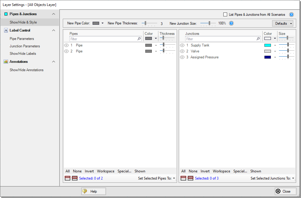
ØOpen the Layer Settings window for the All Objects Layer by double-clicking the All Objects Layer, clicking the gear icon to the right of the layer name, or selecting the layer and clicking the single gear icon on the Layers Toolbar. The Layer Settings window is shown in Figure 39.
The Layer Settings window provides flexible options for customizing the appearance of the model. The Pipes & Junctions group allows you to show or hide junctions, and change display properties like color, size, and thickness. Note that you cannot hide individual objects on the All Objects Layer, but you can hide objects on new layers, and then hide the entire All Objects Layer below. The Label Control group allows you to display input and output parameters next to objects on the Workspace. The Annotations group allows you to customize annotations.
-
ØSelect the Pipe Parameters item under the Label Control group. The left pane lists input and output parameters available for display, and the right pane lists the parameters currently being displayed by the layer on the Workspace.
-
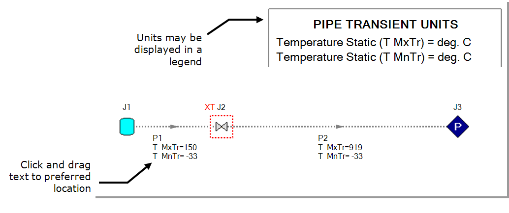
ØIn the left pane, expand the Pipe Max/Min Parameters list. Then, select Max Temperature Static in the list with units of deg.
-
ØAdd additional clarity by repositioning the labels and adding a legend. It is common for the text on the Workspace Layers to overlap with objects when first generated. Labels can be dragged to a new area or a smaller font can be selected using the Font Decrease icon on the Workspace Toolbar or from within the Global Layer Settings. Parameter units can be consolidated in a legend which can be added via the Global Layer Settings. In the Layers Toolbar, click the double gear icon to open the Global Layer Settings. Then, enable the checkbox for Show Units in Legend. The result of these adjustments is shown in Figure 40.
Step 8. Examine the effect of heat transfer
By default AFT xStream models all pipes as adiabatic at the internal surface, meaning no heat is transferred from the fluid to the pipe walls or surroundings. Modeling the pipes as adiabatic is reasonable when the pipes are well insulated and the temperature difference between the fluid and the atmosphere is relatively low. However, for cases such as the tank blowdown modeled in this example, heat transfer from the fluid to the pipe walls and environment has a large impact on results.
-
ØCreate a child scenario named Convective Heat Transfer.
-
ØOpen the Pipe Properties window for each pipe and enter the following on the Heat Transfer tab:
-
Heat Transfer Model = Convective Heat Transfer
-
External Convection Coefficient Correlation = Free-Horizontal (Churchill-Chu)
-
Ambient Temperature =
-
After updating each of the pipes open the Analysis Setup window and go to the Pipe Sectioning and Output panel. Change the Estimated Maximum Pipe Fluid Temperature During Transient to
-
ØRun the model and go to the Output window.
Note that a new caution is shown for heat transfer results in the steady-state. AFT xStream can’t solve for convective heat transfer when there is no flow in a pipe in the steady-state, so xStream treats all stagnant pipes as isothermal at the temperature of the connected boundary junctions. The Temperature Override feature on the Optional tab of the Pipe Properties window can be used to specify a different temperature for the pipe if needed.
In the Transient Max/Min tab shown in Figure 41 it can be seen that the maximum temperature in Pipe P2 is only
Go to the Graph Results window and recreate the Pipe P2 outlet graph from Figure 34 as is shown below in Figure 42.
Step 9. Examine the effect of sectioning
In AFT xStream, sectioning plays an important role in model accuracy. Due to how the MOC operates, accuracy increases with the number of sections you have in the model. To illustrate this, the model was re-run with a Minimum Number of Sections Per Pipe of 6 instead of 1. Comparing Figure 36 to Figure 45, values such as the temperature and pressure for Tank J1 remain similar with the increase in the number of sections. However, values such as the maximum temperature reached in Pipe P2 (Figure 26 and Figure 43), changed substantially. This value increased from
Due to the long run time, it was not sensible to ask you to run the 6 section scenario as a part of this example. If you are interested, you may want to run this scenario overnight.
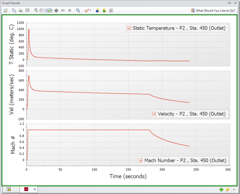
Figure 44: Temperature, velocity, and Mach number for the discharge of Pipe P2 with 6 sections minimum per pipe
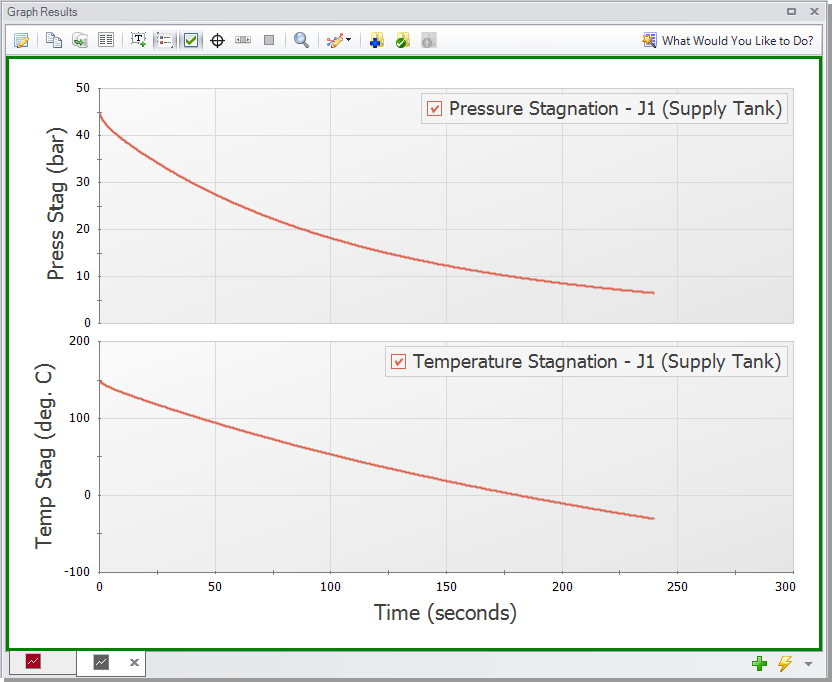
Figure 46: Profile Graph for Tank Blowdown system with 6 Sections Minimum Per Pipe
Conclusion
You have now used the Primary Windows in AFT xStream to build and analyze a simple gas transient model. Pipes and junctions were placed on the Workspace and defined by entering data into their Properties windows. Analysis Setup was used to select a fluid, section the pipes, and enter a duration for the transient simulation. The model was run and results were viewed in the Output window. Different types of graphs were created to analyze the system behavior, and the effect of sectioning was discussed.


