Fluid Library Comparison - Steam Turbine Shutdown Example (Metric Units)
For the US units version of this example, click here.
Two turbines in a high pressure steam system are simultaneously shut down while a bypass line is opened. Evaluate the maximum pressure at the turbine inlets. Additionally, quantify the mass flow rate through the bypass valve throughout the transient and perform an analysis on whether condensation or two-phase flow occurs in the bypass line. Lastly, conduct a sensitivity analysis based on the selection of different fluid library data.
Topics Covered
-
Using the isometric grid to create a model
-
Modeling a transient turbine shutdown
-
Creating transient graphs
-
Animating profile graphs
-
Evaluating the selection of a fluid library
Required Knowledge
This example assumes that the user has some familiarity with AFT xStream such as placing junctions, connecting pipes, and entering pipe and junction properties. Refer to the
Model File
A completed version of the model file can be referenced from the Examples folder as part of the AFT xStream installation:
C:\AFT Products\AFT xStream 3\Examples
Step 1. Build the model
A. Place the pipes and junctions
Isometric Drawing Mode
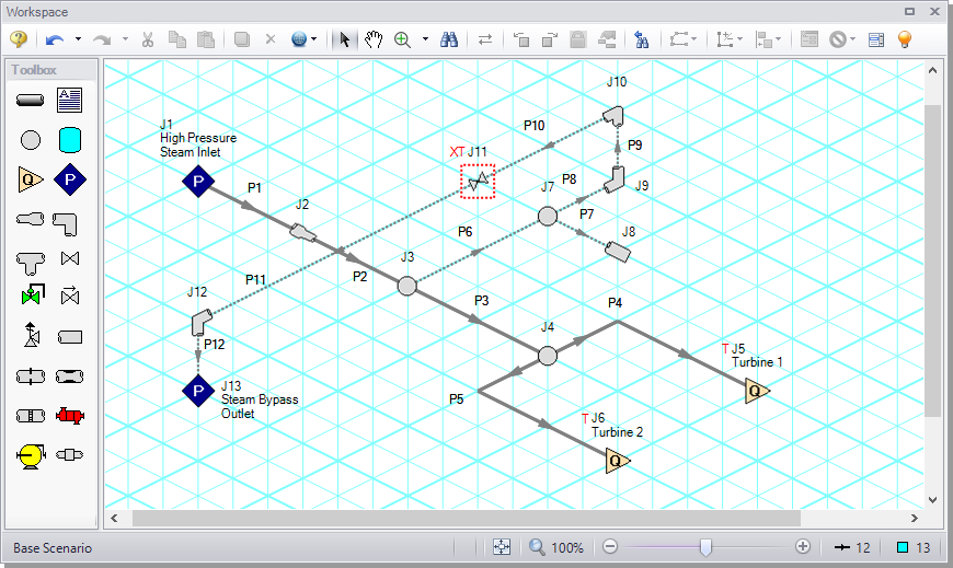
The previous example models were drawn using the default Pipe Drawing Mode, 2D Freeform. AFT xStream has two additional available drawing modes, 2D Orthogonal and Isometric. In this model, the isometric mode is used to visually interpret the pipe layout and provide a better understanding of the system.
-
Open the Arrange menu again, go to Pipe Drawing Mode, and select Isometric.
-
Place the junctions as shown in Figure 1.
-
Click the Pipe Drawing Tool and draw the pipes in the model as shown. When drawing segmented pipes such as P5, a red dashed preview line will show how the pipe will be drawn on the isometric grid. As you are drawing a pipe, you can change the preview line by clicking any arrow key on your keyboard or scrolling the scroll wheel on your mouse.
-
Use the Rotate Icons buttons on the Workspace Toolbar, or right-click on the junction and select the Auto-rotate option to automatically align the junction with the connected pipes. Alternatively, Customize Icon can be selected from the right-click menu to manually choose an icon/orientation.
-
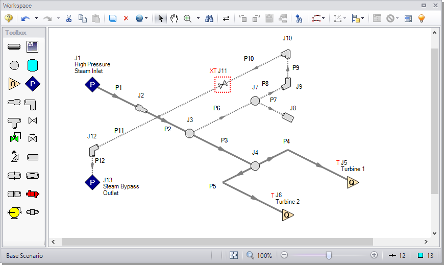
The grid can be shown or turned off in the Arrange menu, as shown in Figure 2.
Note: You can hold the "Alt" key while adjusting a pipe by the endpoint to add an additional segment. This can be used with the arrow key or mouse scroll wheel to change between different preview line options.
B. Enter the pipe and junction data
The system is in place but now the input data for the pipes and junctions needs to be entered. Double-click each pipe or junction and enter the following data in the Pipe or Junction Properties window.
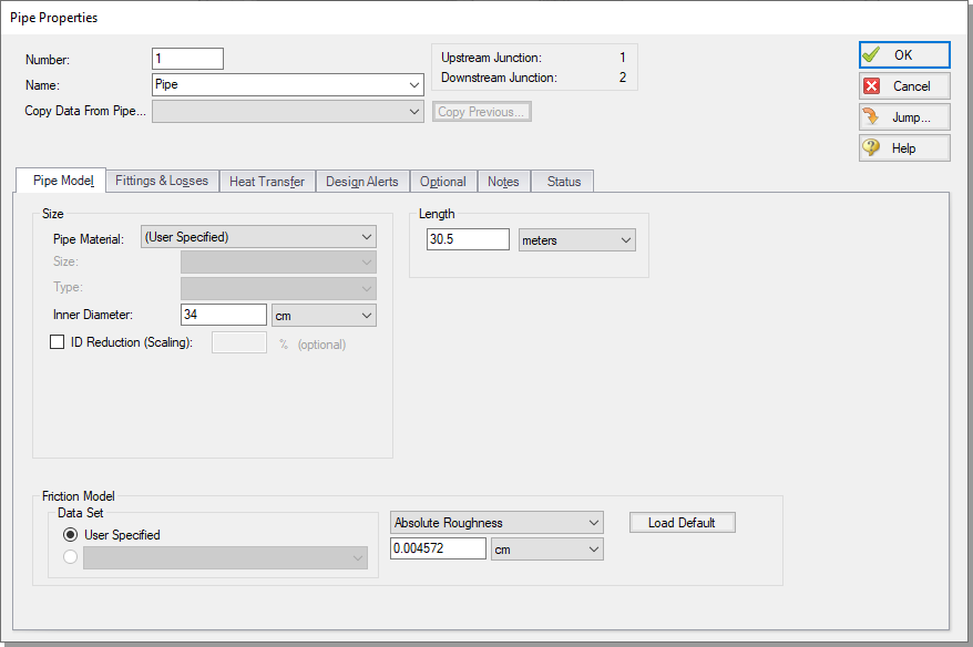
All pipe materials are User Specified in this model (see Figure 3). Use the Absolute Roughness of Steel (
Note: The pipes below are user defined as they utilize non-standard pipe sizes.
| Pipe # | Inner Diameter (cm) | Length (meters) |
|---|---|---|
| 1 | 34 | 30.5 |
| 2 | 30.5 | 20 |
| 3 | 30.5 | 15 |
| 4 | 30.5 | 4.5 |
| 5 | 30.5 | 4.5 |
| 6 | 15.5 | 2 |
| 7 | 10 | 2 |
| 8 | 15.5 | 3 |
| 9 | 15.5 | 1.5 |
| 10 | 15.5 | 6 |
| 11 | 49 | 6 |
| 12 | 49 | 1.5 |
-
Assigned Pressure J1
-
Name = High Pressure Steam Inlet
-
Elevation =
-
Static Pressure =
-
Temperature =
-
-
Area Change J2
-
Type = Conical Transition
-
Angle = 45 degrees
-
-
Branches J3, J4, and J7
-
Elevation =
-
-
Assigned Flows J5 and J6
-
J5 Name = Turbine 1
-
J6 Name = Turbine 2
-
Elevation =
-
Mass Flowrate =
Note: Be advised that the unit for mass flow is not the default, it is
-
Temperature =
-
-
Dead End J8
-
Elevation =
-
-
Bend J9
-
Elevation =
-
Type = Standard Elbow (knee, threaded)
-
-
Bend J10, J12
-
Elevation =
-
Type = Standard Elbow (knee, threaded)
-
-
Valve J11
-
Kv = 2600
-
xT = 0.7
-
Elevation =
-
On the Optional tab, set the Special Condition to Closed
-
Click on the Transient Tab and enter the following data:
-
| Time (seconds) | Kv | xT |
|---|---|---|
| 0 | 0 | 0.7 |
| 2 | 2600 | 0.7 |
| 5 | 2600 | 0.7 |
-
Assigned Pressure J13
-
Name = Steam Bypass Outlet
-
Elevation =
-
Static Pressure =
-
Static Temperature =
-
C. Check if the pipes and junctions are defined
-
ØClick the List Undefined Objects button to see if the model is fully defined. If it is not, the undefined pipes and junctions window will show a list of incomplete items. If undefined objects are present, go back to the incomplete pipes or junctions and enter the missing data.
Step 2. Specify Analysis Setup
A. Specify the Fluid panel
-
ØOpen the Analysis Setup window from the Common Toolbar and open the Fluid panel.
-
ØSelect Steam from the AFT Standard fluid library, and click the Add to Model button.
B. Specify the Pipe Sectioning and Output panel
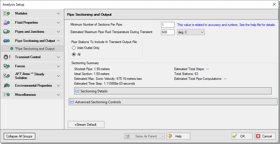
Figure 4: Pipe Sectioning and Output panel
C. Specify the Simulation Mode/Duration panel
-
ØEnter a Stop Time of 5 seconds on the Simulation Mode/Duration panel from the Transient Control group. Verify the Time Simulation is set to Transient. Click the OK button.
Step 3. Run the model
-
ØClick the Run Model button on the Common Toolbar or select the option from the Analysis menu. AFT xStream will prompt you to save the model if you have not done so already, then will open the Solution Progress window.
Step 4. Graph the results
A. Graph the transient pressures at the turbines
-
ØGo to the Graph Results window. The first graph we will make will show the Static Pressure at the entrance to the steam turbines.
-
From the Graph Control tab on the Quick Access Panel, select the Transient Pipe tab
-
Select the Pipe P5 outlet station
-
Ensure that the Time Units are set to seconds
-
Select Pressure Static with units of
-
Click Generate
This will generate the graph shown in Figure 6. The pressure variation is difficult to see using the default y-axis scale so we will adjust the scale using the following steps:
-
Right-click the y-axis
-
Un-check the Auto Scale box
-
Set the Minimum to
The graph should now match Figure 8. When the model contains multiple transient events, transient pipe graphs allow the user to see the cumulative impact of the events on system pressure. Note that the first peak contains an oscillation, which is attributable to the opening of the bypass valve.
![]()
Figure 5: Graph Parameters for the inlet pressure to the turbines
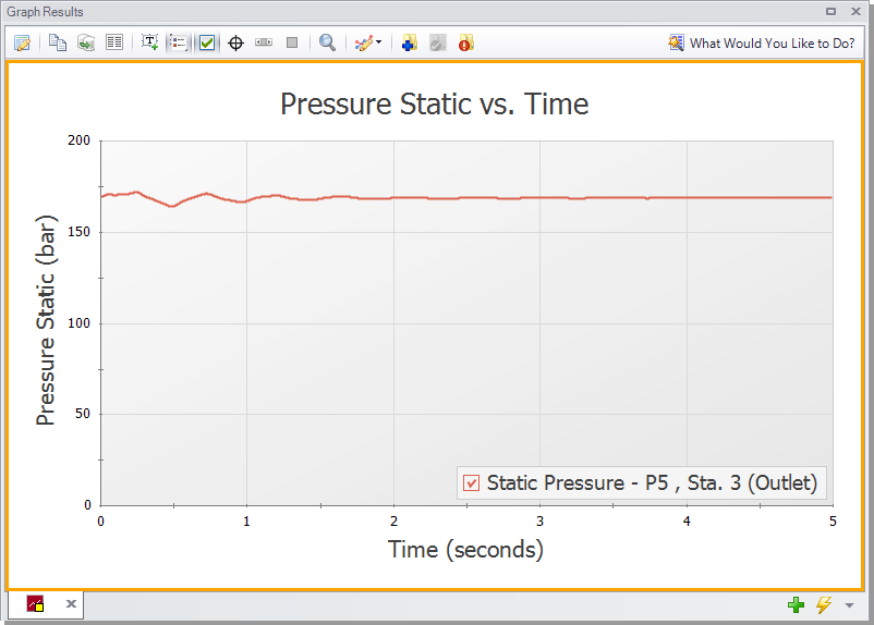
Figure 6: Static pressure at steam turbine 2 entrance
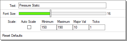
Figure 7: Axis Modification Window opened by right-clicking the y-axis
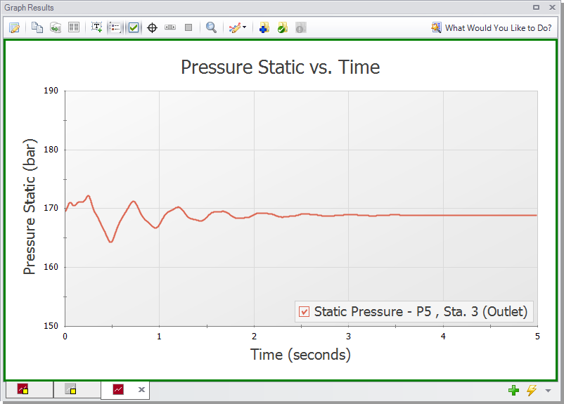
Figure 8: Static pressure at steam turbine 2 entrance with modified y-axis
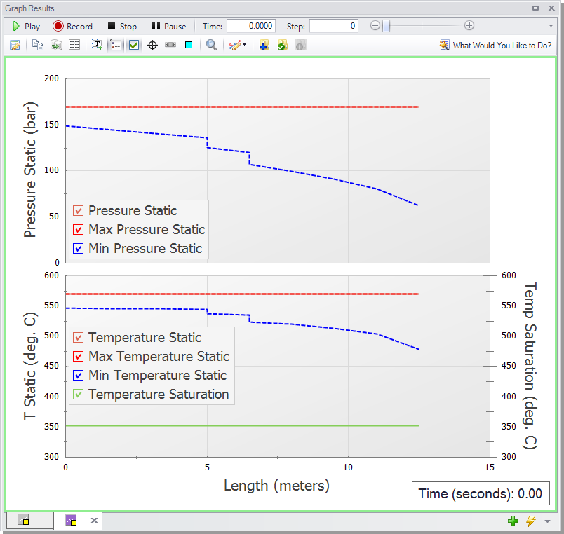
B. Animate the bypass line temperature and pressure
We will also animate the profile of the bypass line temperature and pressure in order to determine whether condensation occurs.
-
Create a new graph tab by clicking the New Tab button located in the bottom-right (green “+” icon).
-
Select the Profile tab under the Graph Control tab in the Quick Access Panel.
-
Select pipes 6, 8, 9, and 10.
-
Verify the Length Units are set to
-
Select the option to Animate Using Output. To use this feature, data from all pipe stations must be saved (which is the default on the Pipe Sectioning and Output panel), otherwise the option will be grayed out.
-
Ensure that the Animation Time Units are set to seconds.
-
Add two additional parameter using the Add button, and specify the three parameters:
-
Pressure Static with units of
-
Temperature Static with units of deg.
-
Temperature Saturation with units of deg.
-
-
Make Temperature Saturation a secondary axis parameter by double-clicking in the empty box to the left of the name. Alternatively, select the parameter and click the right facing blue arrow above the list of parameters. If done successfully, the Temperature Saturation parameter should appear indented under Temperature Static.
-
Uncheck the Mx and Mn boxes only for the Temperature Saturation parameter.
-
Click the Generate button.
-
Adjust the y-axis scaling for both Temperature Static and Temperature Saturation as follows:
-
Right-click on the temperature y-axis and uncheck the Auto Scale box
-
Set the Minimum to
Important: Ensure both the primary (left) and secondary (right) y-axes have the same max and min limits when both parameters have the same unit. This allows for easy visual comparison of the parameters.
-
-
Click the Play button to review the animation. The animation speed can be increased by using the Speed Slider at the right side of the playback controls.
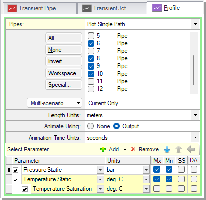
Figure 10 is useful to determine whether or not condensation occurs in the system. Condensation can occur by a rise in pressure, a decrease in temperature, or a combination of both. Each fluid library contains saturation line data and warning messages will be given in the Output if the fluid properties drop into the two-phase region. In this model the temperatures stay well above the saturation line at all times, showing that the steam is not close to condensing.
Reminder: AFT xStream assumes all gases are superheated and does not model two-phase flow. Saturation data is only used for predicting the presence of saturation conditions, and the fundamental equations in the Solver assume the gas is single phase.
C. Graph the mass flow rate and pressure drop through the bypass valve
Lastly, we shall create a graph to show the mass flow rate and the pressure drop through the bypass valve to gain insight into how the flow develops in the bypass line.
-
Create a new graph tab.
-
From the Graph Control tab on the Quick Access Panel, select the Transient Jct tab.
-
In the Select Junctions section, select J11 and click the “>” arrow.
-
Add a second parameter in the Select Parameters section, and specify the two parameters:
-
Mass Flow Rate Inlet with units of
-
Pressure Drop Stagnation Total with units of
-
-
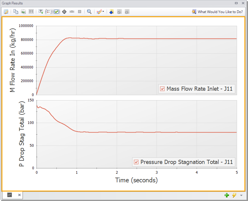
Click the Generate button.
As shown in Figure 12, the flow rate increases and the pressure drop decreases as the valve opens over time. While the observed trends for mass flow rate and pressure drop are typical for a valve that is opening, it is still worthwhile to make Transient Jct graphs when multiple transient events occur in order to fully understand the interactions between them.
Note:Figure 12 has modified axes titles and its legend removed for clarity.
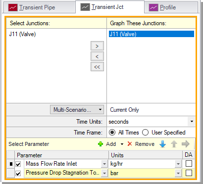
Figure 11: Graph Parameters for the Bypass Valve mass flow and pressure drop
Step 5. Evaluate the effects of changing fluid libraries
A. Review the results of other libraries
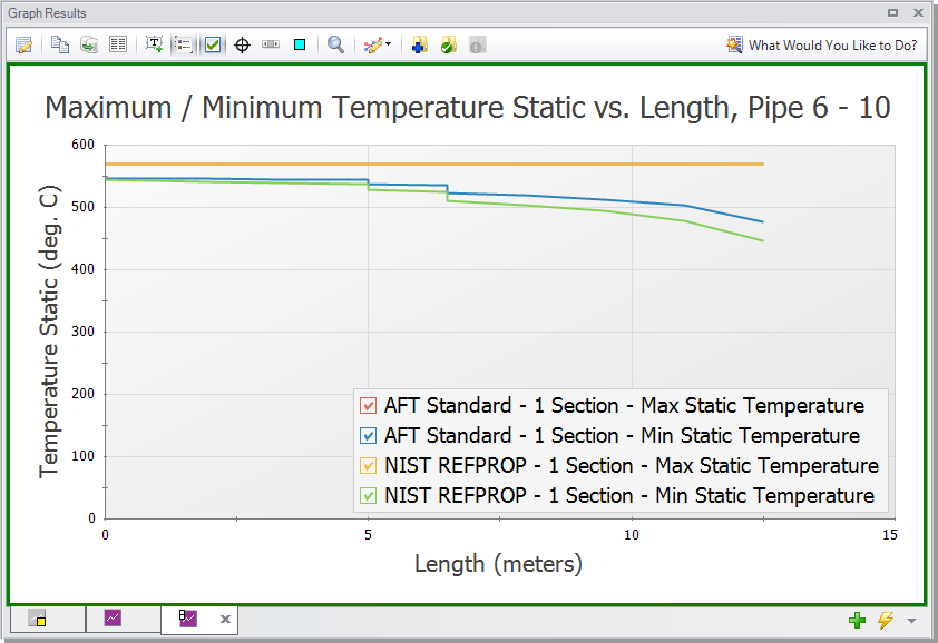
In addition to the AFT Standard fluid library, the model built in this example was run using Steam from the Chempak, NIST REFPROP, and ASME Steam libraries. Similar results to the AFT Standard fluid run were obtained for both the bypass valve and the turbine pressure vs time graph, so these results are not shown below. Nevertheless, it is sensible to run your system using different fluid libraries as they have been known to impact results. The temperature profile for the bypass line showed more significant differences, as is shown below comparing the results using NIST REFPROP vs AFT Standard (Figure 13). ASME Steam and Chempak gave nearly identical results to NIST, and therefore are not shown.
Note that the minimum temperature reached at J11 is about
B. Advice for preliminary runs
Obtaining final results from AFT xStream will require multiple iterations. To effectively work through those iterations, we recommend the iterative process begins with the following steps:
Step 1: Run the steady-state model with multiple fluid libraries
It is recommended that the first runs are completed using a simplified version of your model in the AFT Arrow™ Steady-State Solver with each fluid property model before considering transient conditions. This will allow for larger issues in the model to be caught before having to commit to Transient runs, which are more time consuming. This also can inform the types of variables that need to be considered during refined runs (i.e. if the AFT Arrow™ steady-state runs are close to the saturation temperature, condensation is a phenomenon that should be monitored in subsequent runs).
Step 2: Complete a transient run using an AFT Standard fluid with minimal sectioning
You should then run your simplified model in the Transient Solver using an AFT Standard fluid with minimal sectioning (i.e. a lower value for the Minimum Number of Sections Per Pipe setting on the Pipe Sectioning and Output panel in Analysis Setup). This is not always possible, such as when mixtures are present, but this step should always be attempted if allowable. This will allow for larger issues to be caught before committing to extended run times. Only after you are satisfied with the model should you attempt increasing the number of sections.
C. Selection of fluid property model for final runs
A number of factors must be taken into consideration while selecting the fluid library for an AFT xStream model. If there are no mixtures, and the compound is present in the AFT Standard library, it is recommended that the AFT Standard library be the first library used. AFT Standard has the shortest run times of the different libraries and is an excellent choice for early runs focused on troubleshooting the model. However, if there is a need to model mixtures, and simplifying the system is not possible, initial runs should be conducted with NIST REFPROP or Chempak.
NIST REFPROP and Chempak both have greater accuracy than AFT Standard and can model mixtures. However, both have slower run times than AFT Standard. Chempak typically runs faster than NIST REFPROP with comparable accuracy. However, Chempak is an optional add-on for purchase while the NIST REFPROP library comes standard with AFT xStream.
Lastly, ASME Steam provides a well-established, trustworthy source of steam data. ASME Steam typically has the longest run times, and it is recommended that a high processing power computer paired with ample time be used to run your analysis if this library is selected. If either of those elements are unavailable, it is recommended that one of the other libraries be used, with the added note that NIST REFPROP is the most similar in accuracy to ASME Steam.
Table 1 summarizes the run times for this example with the different fluid libraries. The run times will be affected by the specifications of your computer as well as the memory available. Table 1 shows data for runs conducted on the laptops at AFT as of publication.
Additionally, Table 2 provides a library compatibility chart to assist with fluid property model selection.
It should be noted that if a tremendous amount of accuracy is needed, appropriate library selection will not be sufficient to give a high accuracy model. The single parameter that will have the greatest effect on accuracy is the Minimum Number of Sections per Pipe in the Sectioning panel. Ultimately, appropriate sectioning remains the single most important factor in creating a high accuracy model and should be weighed just as heavily as the fluid library when setting the parameters your transient gas system uses.
Table 1: Comparison of run times with various fluid libraries
| Steam Turbine Shutdown Approx Run Times | |
| Fluid Property Model | Run Time |
| AFT Standard - 1 Section | 2 - 3 minutes |
| Chempak - 1 Section | 4 - 10 minutes |
| NIST REFPROP - 1 Section | 0.9 - 1.4 hours |
| AFT Standard - 10 Sections | 1 - 2 hours |
| ASME Steam - 1 Section | 3 - 4 hours |
Table 2: Compatibility chart for fluid library selection for final runs
| Fluid Library | Model Requirements | ||||
|---|---|---|---|---|---|
| Mixtures | Condensation Data | System Troubleshooting | Final Runs | Complex Systems |
|
| AFT Standard | ✔ | ✔ |
✔ | ||
| NIST REFPROP | ✔ | ✔ | ✔ | ✔ | |
| Chempak | ✔ | ✔ | ✔ | ✔ | |
| ASME Steam | ✔ | ✔ | |||
* Evaluating the complexity of a system is most easily done in early runs of the model. It is suggested that all early runs should be run with a version of AFT Standard if they can, and the run time recorded. This run time should inform your decision on which fluid library is needed to run the more thorough runs when high accuracy results are needed. As seen from Table 1, the run times can vary wildly between the 4 libraries, so make sure you evaluate your time constraints and accuracy needs when weighing this decision. Factors that can impact the run time include the ratio in the length of the smallest pipe to the largest pipe, presence of mixtures, usage of Junctions containing resistance curves, and the presence of sonic choking. See the Reducing Run Time section for more information.
** It is strongly recommended that all runs used to troubleshoot the design of the system are run using AFT Standard.
Conclusion
Graphs were created showing the turbine inlet pressure over time, and animating the pressure and temperature in the bypass line. It was determined that no condensation occurs, regardless of which fluid library was used.
A standard procedure for initial and final runs was discussed:
-
Step 1: Run the steady-state model with multiple fluid libraries
-
Step 2: Complete a transient run using an AFT Standard fluid with minimal sectioning
Lastly, a comparison of the different fluid libraries was discussed. AFT Standard should be used for initial runs and troubleshooting (runs faster). NIST REFPROP, Chempak, and ASME Steam libraries should be used for final runs where higher accuracy is required; however, the trade off is that the model will have significantly longer run times.


