Frequency Analysis - PFA Example
(Metric Units)
For the US units version of this example, click here.
The preliminary design for a system uses a positive displacement reciprocating compressor that is single-acting and has two heads (cylinders) with a 180 degree phase offset. It is suspected that the design may have pulsation resonance issues and needs to be checked for compliance with the API 618 standard. Perform a frequency analysis by placing a forcing function on the PD compressor and observing the frequency response of the system. Determine the worst acoustic natural frequency of the system, run the compressor at the worst-case RPM, and determine if the API 618 limits are violated.
Topics Covered
-
Using the PFA Module to identify natural acoustic frequencies
-
Defining valid sectioning and simulation duration settings for pulsation analysis
-
Identifying problematic compressor speeds based on pulsation frequency and cylinder arrangement
-
Using periodic flow to represent a reciprocating compressor
Required Knowledge
This example assumes that the user has some familiarity with AFT xStream such as placing junctions, connecting pipes, and entering pipe and junction properties. Refer to the
Model File
A completed version of the model file can be referenced from the Examples folder as part of the AFT xStream installation:
C:\AFT Products\AFT xStream 3\Examples
Step 1. Activate the PFA module
Open the Analysis Setup window and go the Modules panel under the Modules group. Then, select the option to Activate PFA.
Step 2. Build the model
A. Place the pipes and junctions
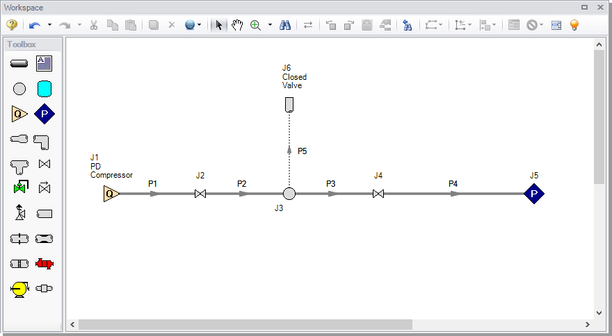
The next step is to define the pipes and junctions. In the Workspace window, assemble the model as shown in Figure 1.
B. Enter the pipe and junction data
The system is in place but now we need to enter the input data for the pipes and junctions. Enter the following data:
All Pipes are Steel - ANSI, STD (schedule 40), and have standard roughness. The rest of the pipe information is as follows:
| Pipe # | Length (meters) | Size (inches) |
|---|---|---|
| 1 | 8 | 10 |
| 2 | 8 | 10 |
| 3 | 8 | 10 |
| 4 | 80 | 16 |
| 5 | 3 | 6 |
-
Assigned Flow J1
-
Elevation =
-
Name = PD Compressor
-
Mass Flow Rate =
Note: This is the average bulk flow produced by the compressor.
-
Temperature =
-
-
Valve J2
-
Elevation =
-
Loss Source = User Specified
-
Loss Model =
-
-
xT = 0.8
-
-
Branch J3
-
Elevation =
-
-
Valve J4
-
Elevation =
-
Loss Source = User Specified
-
Loss Model =
-
-
xT = 0.6
-
-
Assigned Pressure J5
-
Elevation =
-
Stagnation Pressure = 0
-
Temperature =
-
-
Dead End J6
-
Elevation =
-
Name = Closed Valve
-
C. Check if the pipe and junction data is complete
-
ØTurn on List Undefined Objects from the Main Toolbar to verify if all data is entered. If it is not, the undefined pipes and junctions window will show a list of incomplete items. If there are undefined objects, go back to the incomplete pipes or junctions and enter the missing data.
Step 3. Specify Analysis Setup
A. Fluid panel
-
ØOpen the Analysis Setup window and select the Fluid panel under the Fluid Properties group.
-
ØSelect Methane from the AFT Standard fluid library, and click the Add to Model button.
B. Pipe Sectioning and Output panel
C. Simulation Mode/Duration panel
-
ØEnter a Stop Time of 2 seconds on the Simulation Mode/Duration panel in the Transient Control group.
D. Pulse Setup panel
-
ØOpen the Pulse Setup panel from the Pulsation Setup group. The Pulse Setup panel is used to specify the location and magnitude of the pulse applied to the system, as well as the parameters required to generate the forcing function for frequency analysis.
-
ØDefine the Pulsation inputs as follows (Figure 2):
-
Select Natural Frequency Evaluation for the Frequency Analysis Mode.
-
Select junction J1 as the location for the pulse to be applied at.
-
For Magnitude, ensure that Automatic (Twice Steady-State Flow) is selected.
-
Under Frequency Analysis, define the Cutoff Frequency as 200 Hz and verify that the Minimum Number of Frequency Samples is set to the default value of 1000.
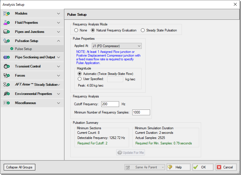
Now that all of the pulsation inputs are defined, look at the Pulsation Summary at the bottom of the window. The defined Cutoff Frequency and the Minimum Number of Frequency Samples will affect the number of sections and the simulation duration that are required to run the analysis. If the number of sections is insufficient, then the time step will be too large to capture the specified Cutoff Frequency. Similarly, if the simulation duration is too small, then the number of time steps will not accommodate the Minimum Number of Frequency Samples.
Checking the Pulsation Summary for this example, the Minimum Sections Required for Cutoff are 2, and the Minimum Simulation Duration Required for Min. Samples is
Step 4. Run the model
-
ØSelect Run Model from the Common Toolbar. This will open the Solution Progress window. This model has an estimated run time of 5 minutes, but the run time is dependent on the speed of your PC.
Step 5. Ensure the pressure response stabilizes
-
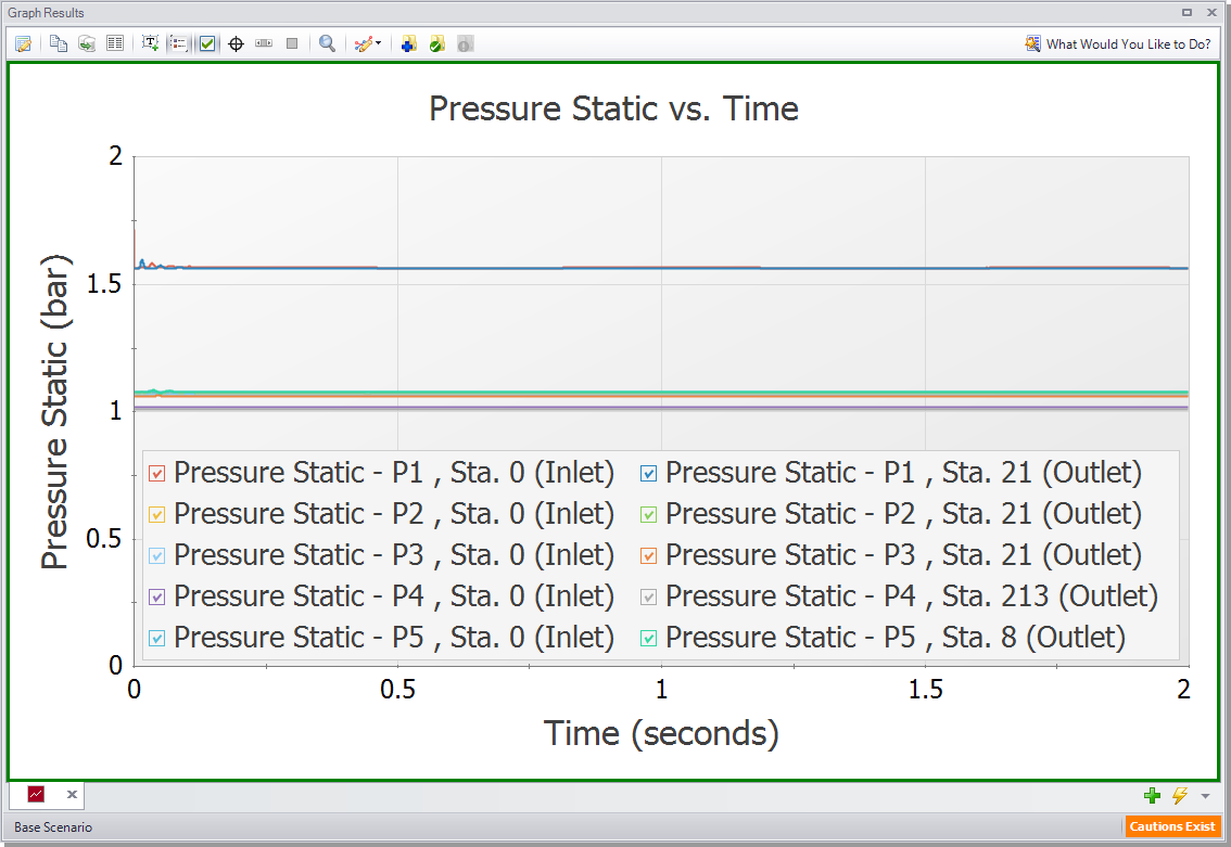
ØOpen the Graph Results window. The first step will be to generate a plot of the pressure in each of the pipes to ensure that the simulation duration was long enough for the response to stabilize.
-
ØCreate the pressure graph as follows:
-
Select the Transient Pipe tab from the Graph Control tab of the Quick Access Panel
-
Add the Inlet and Outlet station for each of the pipes
-
Choose Pressure Static as the Parameter in units of
-
Click Generate
The pressure graph should appear as shown in Figure 3. Note that there is a small perturbation in the pressure when the pulse is applied to the system, though the pressure results completely stabilize by the end of the run. If the pressure results were still changing at the end of the run, the model should be re-run with a longer simulation duration.
Step 6. Graph the frequency response
-
ØNext, graph the acoustic frequency response as follows:
-
Click the New Tab button (green “+” icon in the bottom-right)
-
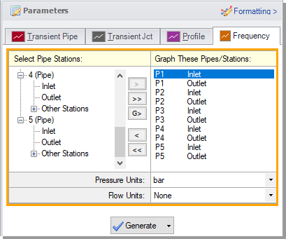
Select the Frequency tab in the Graph Parameter section of the Quick Access Panel (Figure 4)
-
Add the Inlet and Outlet station for each of the pipes
-
Verify that the pressure units are set to
-
Click the Generate button
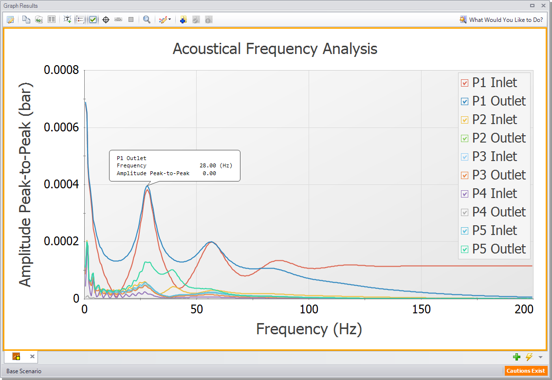
Identify excitation frequencies to study
From the graph in Figure 5, there are several frequencies that produce a large pressure response. Points on the plot with a large response magnitude are easily identified by finding local maxima on the graph. The frequency and amplitude associated with these maxima can be highlighted on the graph by clicking and dragging the cursor from left to right highlighting the location of the local maximum. These maxima are the acoustic natural frequencies that are potentially the most damaging when excited by a positive displacement compressor. These frequencies can also be caused by equipment that contributes large pressure drops, such as control valves.
Two natural frequencies are identified for the system based on the peaks in the graph at roughly
Step 7. Simulate the worst-case scenario
A. Determine the worst-case RPM
The

In this case
B. Create a scenario with Steady State Pulsation
-
ØCreate a child scenario and switch to Steady State Pulsation analysis mode:
-
In the Scenario Manager, right-click on the Base Scenario and choose Create Child. Name the child scenario “
-
Open the Analysis Setup window and go to the Pulse Setup panel.
-
Switch the Frequency Analysis Mode to the Steady State Pulsation option.
-
Under the Pulsation Source section, select the Reciprocating Compressor option. The Compressor dropdown menu will show User Defined since this example is using an Assigned Flow junction to represent the discharge of the compressor.
-
Enter the Speed as
-
Ensure the checkbox for Evaluate with API 618 is enabled. Click OK to save and close Analysis Setup.
C. Approximate the compressor flow
Since the PD compressor is single-acting and has 2 compression cylinders with a 180 degree phase offset, we can take advantage of the Periodic Flow option in the Assigned Flow junction to create a modified sine wave that approximates the mass flow leaving the compressor. In this case, having 2 heads with a 180 degree offset results in an easy, symmetrical chopped sine wave with two peaks per period.
The Periodic Flow with Chopped Sine Wave option will require a frequency and amplitude. For the Chopped Sine Wave sub-option, the frequency represents two peaks. It is equivalent to taking the absolute value of a full period of a normal sine wave. Assuming that the minimum flow that occurs between the peaks is zero, the flow amplitude must scale the steady-state flow rate by π/2 to achieve an equivalent bulk flow rate. This is shown in Figure 6 for one crankshaft rotation, and the areas under the steady-state and periodic mass flow curves are equal to the other. This scaling results in a flow amplitude of
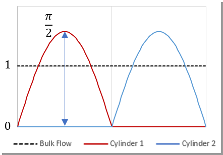
Figure 6: Illustration of transient and steady mass flow rates with identical areas under the curves, resulting in equivalent bulk flow rates
-
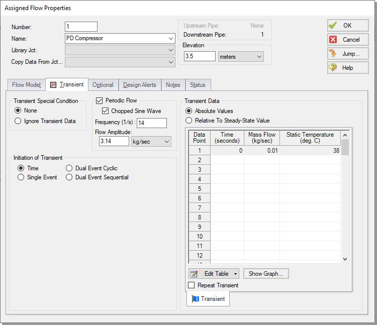
ØModify the Assigned Flow junction to represent steady-state pulsation:
-
Open the Assigned Flow Properties window for junction J1.
-
In the Flow Model tab, set Mass Flow Rate to 0.01
-
In the Transient tab, clear the pulse transient data by clicking Edit Table under the transient table and choosing Clear All Data.
-
Check the boxes next to Periodic Flow and Chopped Sine Wave.
-
Set the Frequency to
-
Set the Flow Amplitude to
-
Click OK to save and close the Assigned Flow Properties window.
The model is now updated to represent the pulsation at the positive displacement compressor that will excite the system.
Step 8. Check for compliance with API 618
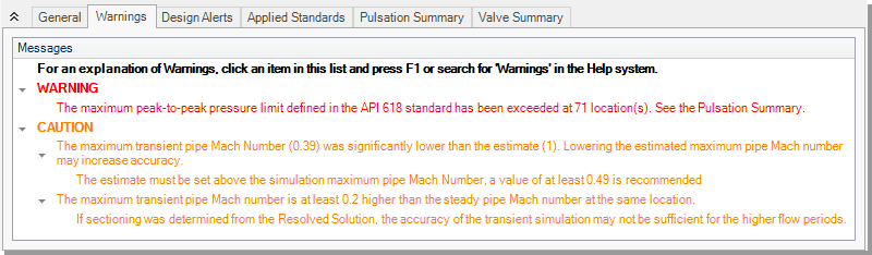
A. Check the Output for warnings
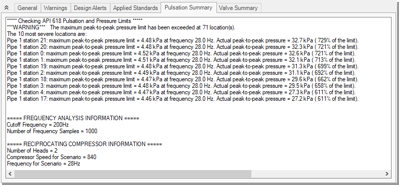
A warning will be shown stating that the maximum pressure limit for API 618 was exceeded as is shown in Figure 8. The caution message stating that lowering the estimated maximum pipe Mach number may increase accuracy is useful for improving sectioning, but iterating on this value is not necessary for the purpose of this example. The caution message about the maximum transient pipe Mach number exceeding the steady pipe Mach number can be ignored, since this is to be expected based on the flow amplitude.
When the API 618 evaluation is performed, the Pulsation Summary tab is shown in the Output window with additional information on where pressure limit violations occurred, and what inputs were used to calculate the API 618 pressure limits for the scenario (Figure 9).
B. Examine the pulsation at the compressor
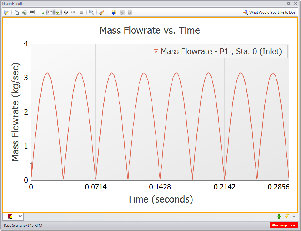
The pulsation behavior at the outlet of the compressor can be illustrated by graphing the flow at the inlet of Pipe P1.
-
Select the Transient Pipe tab in the Graph Parameter section of the Quick Access Panel
-
Add the Outlet station from Pipe P1
-
Select Mass Flowrate as the graphing parameter with units of
-
Ensure that Time Units are set to seconds
-
Click the Generate button
-
Right-click on the x-axis and uncheck the Auto Scale option
-
Set the Maximum to
-
Set the Major Val to
The resulting graph is shown in Figure 10. There should be 8 pulses each with a maximum flow near
C. Graph the API 618 limits
There were many locations within the model where the API 618 limits were exceeded. Since this example focused on the closed valve at the J6 Dead End, we will graph the API 618 limits for this location. The same procedure could be applied for any location in the model.
-
Select the Frequency tab in the Graph Parameter section of the Quick Access Panel
-
Add the Pipe P5 Outlet station
-
Ensure the Pressure Units are set to
-
Click the Generate button
Figure 11 shows the resulting graph in which AFT xStream has overlaid the calculated API 618 limits. A noticeable spike is seen at

Because the peak-to-peak pulsation level recommended by API 618 is exceeded, the system design may need to be changed in order to minimize vibration and maximize system longevity. This could be achieved by changing the compressor selection such as one with more cylinders or replacing the compressor with several smaller capacity compressors. Other approaches may include changing pipe geometry or adding pulsation suppression devices such as acoustic filters, pulsation bottles, finite volume surge tanks, or choking tubes.
Conclusion
The PFA Add-on Module for AFT xStream can be used to apply a pressure pulse to the system in order to identify acoustic frequencies which may result in damage. These frequencies can be used in further pulsation analysis to determine if pulsation mitigation is required. The Steady State Pulsation analysis mode and Assigned Flow junction with a periodic chopped sine wave allowed us to simulate the PD compressor running at a specified RPM.
The piping layout and geometry of the system was found to have an excitation frequency of
The peak-to-peak pressure oscillations were found to violate the API 618 standard. Future modifications would need to be made to the system such as changing the compressor, altering the piping layout, or utilizing pulsation suppression devices.


