Pipe Forces from Turbine Shutdown Example (Metric Units)
For the US units version of this example, click here.
Two turbines in a high pressure steam system have their valves simultaneously shut off, which causes the system to experience transient forces. This example describes how to determine the transient force data for the piping system during the steam flow transient. It also evaluates the effect of varying the time to close the valves on force magnitude. Lastly, this example shows how to export the force results to a force file to use in piping stress software.
Topics Covered
-
Calculating the forces associated with a transient event
-
Using the Scenario Comparison Tool to compare scenarios
-
Exporting force sets to CAESAR II®
Required Knowledge
This example assumes that the user has some familiarity with AFT xStream such as placing junctions, connecting pipes, and entering pipe and junction properties. Refer to the
Model File
A partially completed model file will be utilized as the starting point for this example. A completed version of the model file can be referenced if desired. Both the initial and final model files can be found in the Examples folder as part of the AFT xStream installation:
C:\AFT Products\AFT xStream 3\Examples
Step 1. Open the model file
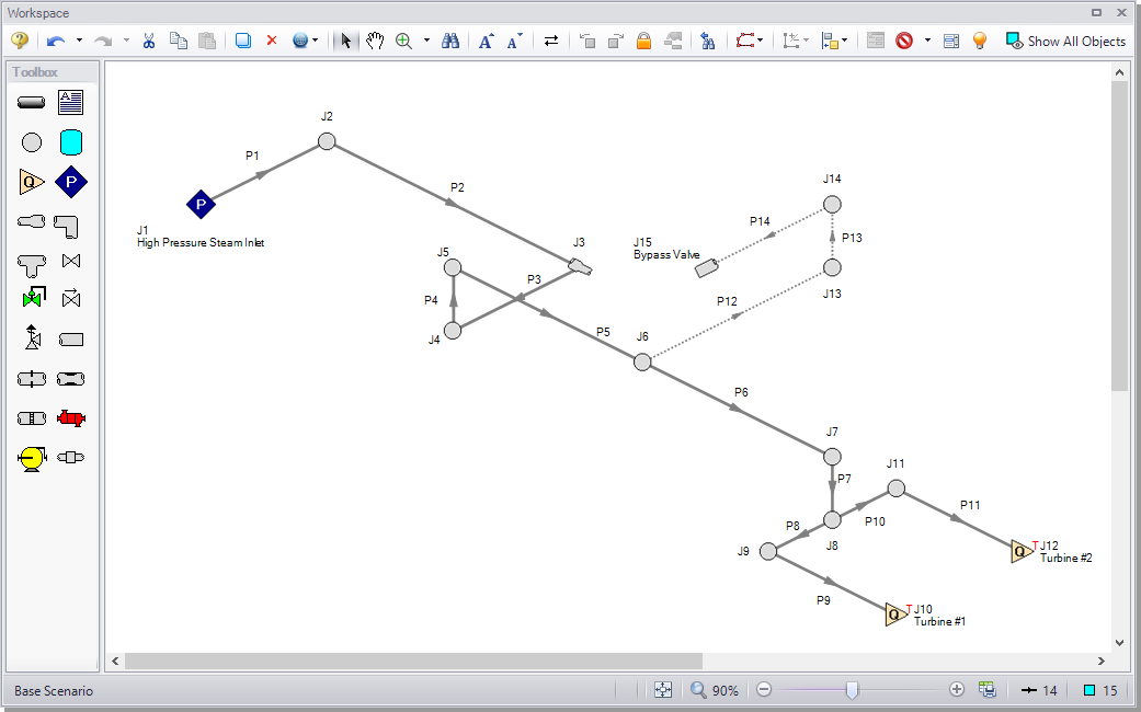
For this example, we will be starting from a pre-built model file which has been partially set up for your convenience. From either the Startup window or the File menu, browse to the model file with the name shown above, using the variant with “- Initial” appended to the file name. The Workspace should appear as shown in Figure 1.
Step 2. Specify the Pipe Sectioning and Output panel
-
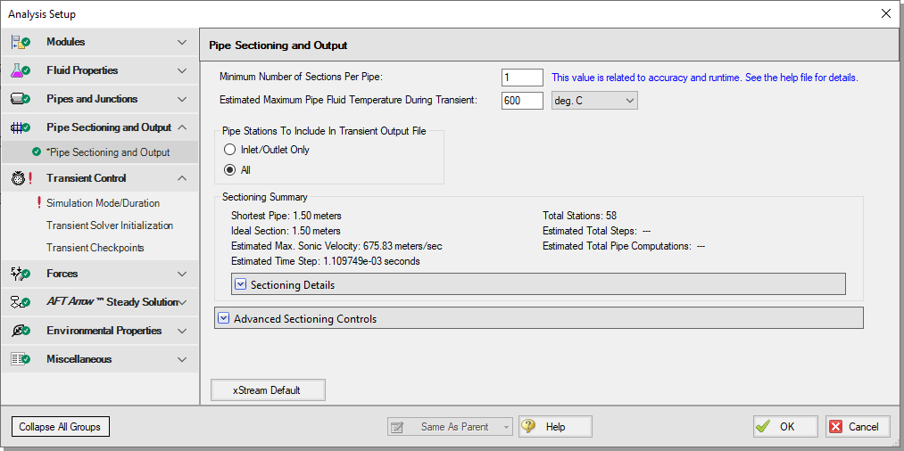
ØOpen the Pipe Sectioning and Output panel in the Analysis Setup window. Define the Minimum Number of Sections Per Pipe as 1 section and the Estimated Maximum Pipe Temperature During Transient as
Step 3. Specify the Simulation Mode/Duration panel
-
ØOpen the Simulation Mode/Duration panel from the Transient Control group. Enter the Stop Time as 1 second. Click OK to save and close the Analysis Setup window.
-
ØOpen the Force Definitions panel from the Forces group.
We will first add one Force Set from the Workspace.
A. Force Types
The Difference force type is intended to model the specific case where all of the following criteria is true:
-
The force is between a pair of 90 degree elbows
-
The force is an axial pipe force
-
All pipes, fittings, and components between the elbow pair are in-line
The force equations in the Solver are specific to this geometry. The pipes and components between the elbow pair can be horizontal, vertical, or sloped, but the axial component of the fluid weight is not accounted for in the forces. AFT xStream only accounts for hydraulic forces, or those acting on the pipe from the fluid. Elevation and hydrostatic pressure are accounted for in the pressure and flow solution.
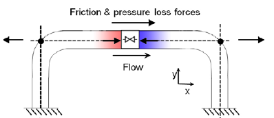
Figure 3: Schematic of the Difference force type
The Point force type would be used for calculating the force at a Dead End junction. It is calculated using the difference in fluid pressure and ambient pressure, multiplied by the pipe area.
The Difference Exit force type would be used between a single 90 degree elbow and a location where the fluid is leaving the system, such as an exit valve, exit orifice, or nozzle.
The force sets in this example will use the Difference force type to calculate the axial forces between 90 degree elbow pairs.
B. Defining Force Sets
Force sets can be defined from the Workspace, or from within Analysis Setup. We will first add one Force Set from the Workspace. Generally it is best to represent each elbow with a unique junction on the Workspace (either an Elbow or Branch). This example assumes that the static pressure loss in the elbows is negligible, and therefore, they are modeled as Branch junctions which are lossless.
-
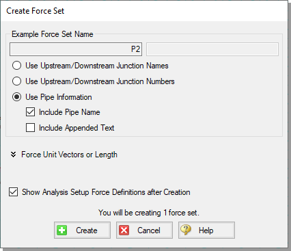
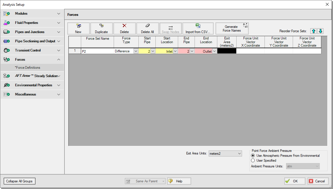
ØOn the Workspace, right-click on Pipe P2 and from the right-click menu select Create a Force Set with Selected Pipe. Select the Use Pipe Information radio button and un-check the Include Appended Text option (Figure 4). Click Create. This will open the Force Definitions panel of the Analysis Setup window. The Force Definitions panel should appear as shown in Figure 5.
AFT xStream can only determine axial forces down a pipe in the direction defined as forward by the force set definition. As such, AFT xStream has no knowledge of the three-dimensional orientation of a given force set. For example, a vertical pipe and a horizontal pipe that both have the same force magnitude would be indistinguishable in AFT xStream. The force set definition informs the sign of the force, with a positive value indicating a force pushing from the start location to the end location, and a negative value indicating the converse.
If a more robust view of the 3D orientation of the pipes is required, directional information can be entered using the optional Force Unit Vector columns. The Force Unit Vectors do not impact AFT xStream's calculations, but may be useful to export the output to piping stress analysis software as discussed in Step 10
Note: Only single pipes can be added as a Difference force set type from the Workspace.
The remaining force sets will be defined inside the Force Definitions panel.
-
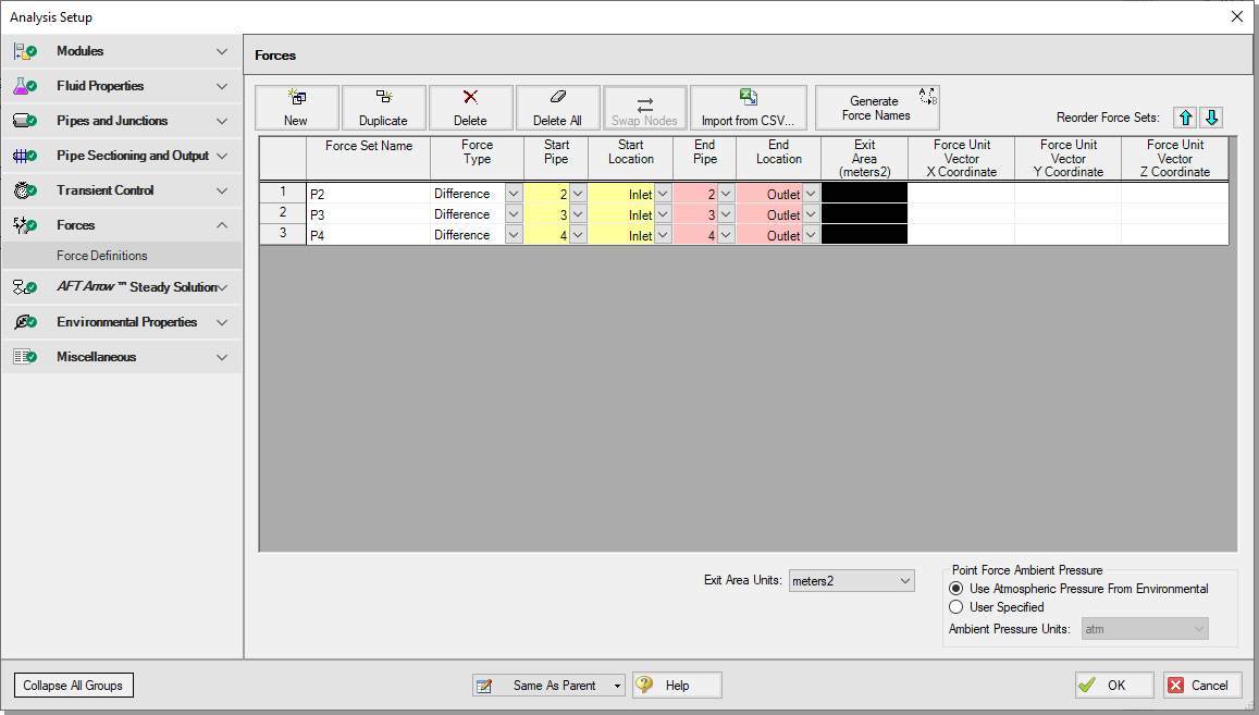
ØDefine a force set by clicking New, selecting the Force Type (in this example, we will be using Difference because all force sets are between 90 degree elbow pairs), entering a name, and defining the starting and ending locations of the force set. Set up the force sets as shown in Figure 6. Click OK to save and close the Analysis Setup window.
-
P2, Difference, P2 Inlet to P2 Outlet (previously created from the Workspace)
-
P3, Difference, P3 Inlet to P3 Outlet
-
P4, Difference, P4 Inlet to P4 Outlet
-
ØDouble-Check Force Set Assumptions: It is important to consider if the force sets adhere to the assumptions mentioned previously which apply to the Difference force type. All of the force sets are located between pairs of 90 degree elbows (represented as lossless Branch junctions). Furthermore, each force set spans a single pipe and there are no branching paths in the middle of the force sets. Therefore, the defined Difference force sets are valid and compatible with the equations programmed into AFT xStream.
Note: A Difference force set that spans Pipes P5-P6 would be between a pair of 90 degree elbows, and would be horizontally in-line; however, it would not be valid since there is a branching flow path in the middle. Even if the flow path from Pipe P12 to the closed bypass valve starts as stagnant in the steady-state, it can be affected by the transient, and could potentially serve as an anchoring support for Pipes P5 and P6. The same applies to Pipe P7, where the Difference force set would not be valid due to the branching flow at the endpoint.
Step 5. Create child scenarios using the Scenario Manager
A. Create scenarios
In this model, we will evaluate three different valve closure durations for the system:
-
0.1 Second Valve Closure
-
0.25 Second Valve Closure
-
0.5 Second Valve Closure
We will create three child scenarios to model the three cases.
-
ØGo to the Scenario Manager on the Quick Access Panel. Create a child scenario by either right-clicking on the Base Scenario and then selecting Create Child, or by first selecting the Base Scenario and then selecting the Create Child icon
 . Enter the name "0.1 Second Valve Closure" in the Create Child Scenario window, and click OK. The new scenario should now appear in the Scenario Manager on the Quick Access Panel below the Base Scenario.
-
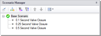
ØRight-click the Base Scenario in the Quick Access Panel. Create another child and call it "0.25 Second Valve Closure". Finally, create one more child and call it "0.5 Second Valve Closure". The child scenarios should now be displayed as shown in Figure 7.
B. Define the child scenarios
Since the "0.1 Second Valve Closure" scenario uses the same transient definitions as the base scenario, we do not need to modify it. Having a duplicate of the parent scenario is useful for organizing Multi-Scenario graph selections and keeping your scenario tree intuitive. We will set up the remaining scenarios using the following steps:
-
Load the "0.25 Second Valve Closure" scenario by double-clicking the name in the Scenario Manager.
-
Open the Assigned Flow Properties window for Assigned Flow J10 and open the Transient tab. Enter the following data:
| Time (seconds) | Mass Flow( |
Static Temperature (deg. |
|---|---|---|
| 0 |
|
|
| 0.25 | 0 |
|
| 1 | 0 |
|
-
Enter the same Transient Data for Assigned Flow J12.
-
Open the Child Scenario "0.5 Second Valve Closure" from the Scenario Manager.
-
Open the Assigned Flow Properties window for Assigned Flow J10 and open the Transient tab. Enter the following data:
| Time (seconds) | Mass Flow( |
Static Temperature (deg. |
|---|---|---|
| 0 |
|
|
| 0.5 | 0 |
|
| 1 | 0 |
|
-
Enter the same Transient Data for Assigned Flow J12.
Step 6. Compare child scenarios using the Scenario Comparison Tool
The three scenarios created should be identical except for the different transient data. To confirm the scenarios are otherwise identical, we will use the Scenario Comparison Tool.
-
Load the "0.1 Second Valve Closure" scenario from the Scenario Manager.
-
In the Tools menu, select the Scenario Comparison Tool.
-
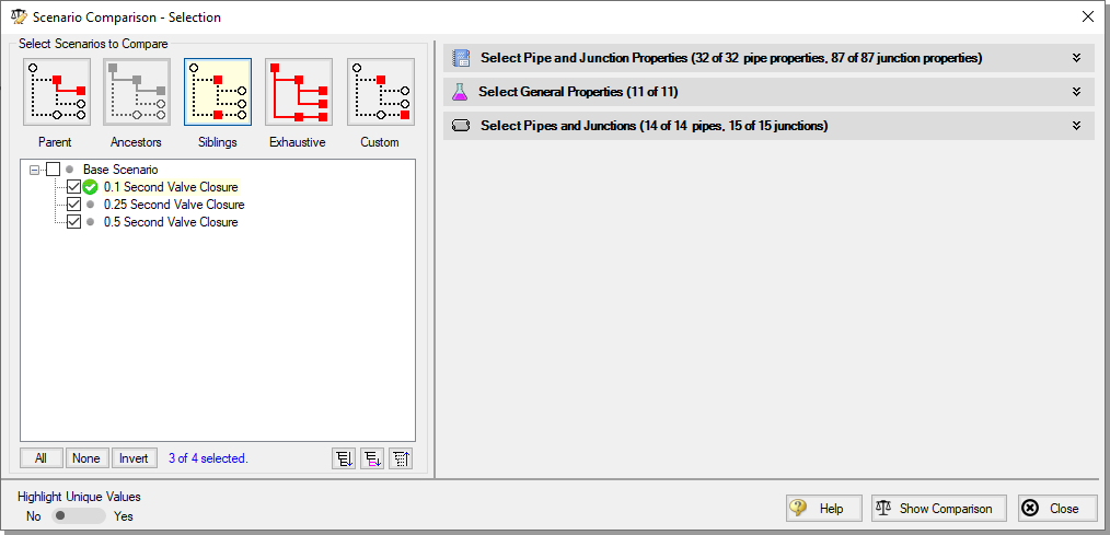
In the Scenario Comparison - Selection window (Figure 8), select the Siblings option.
-
Click Show Comparison.
-
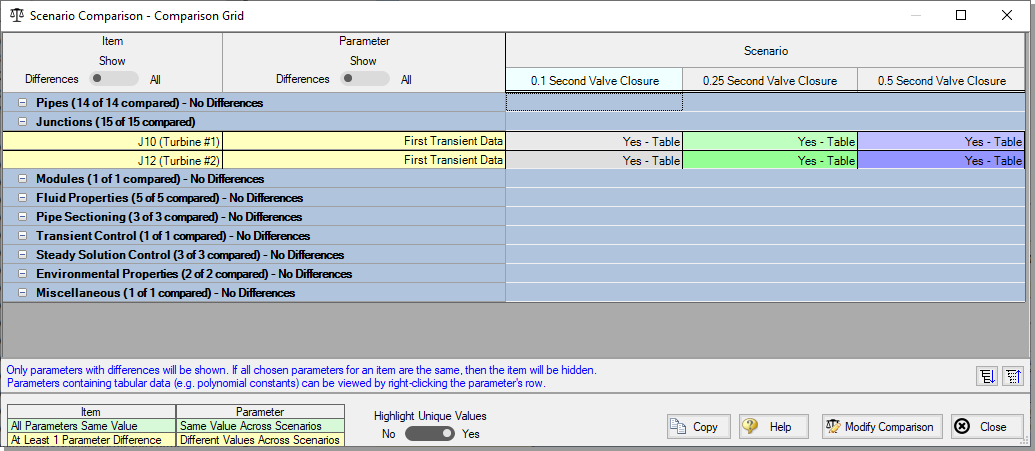
In the Scenario Comparison Grid, set the Item and Parameter sliders to show Differences. Also set the Highlight Unique Values slider to Yes.
The Scenario Comparison Tool will run a comparison of all Pipe and Junction Properties as well as the General Properties used in each scenario and highlight any differences in the Scenario Comparison Grid. In this model, the only highlighted differences should be for the First Transient Data parameter for junctions J10 and J12 (Figure 9). Note that each column in the Scenario Comparison Grid is highlighted in a different color. This indicates that each scenario possesses a unique value for the given parameters. Click close to exit the Scenario Comparison Tool.
Step 7. Run the first scenario
-
ØDouble-click the "0.1 Second Valve Closure" child scenario in the Scenario Manager. Select Run Model from the Analysis menu. This will open the Solution Progress window. Once finished, click Output on the Solution Progress window.
Step 8. View the results
-
ØIn the Output window, click on the Forces tab. This will show the maximum force observed in the defined force sets, as well as provide information about how the force segments were defined.
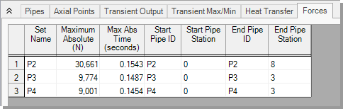
Figure 10: Forces tab in the Output window for the "0.1 Second Valve Closure" scenario
B. Graph the force results
-
ØOpen the Graph Results window. We will create a graph that shows the transient forces over time for the force sets. To do so, perform the following steps:
-
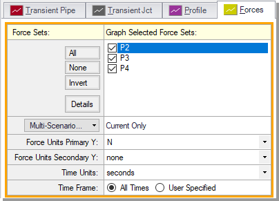
Select the Forces tab on the Graph Control tab on the Quick Access Panel, as shown in Figure 11.
-
Click the All button such that all force sets are selected from the list to be graphed.
-
Verify the Force Units Primary Y is set to
-
Verify that Time Units is set to seconds.
-
Verify that the Time Frame is set to All Times.
-
Click Generate.
This should generate the graph shown in Figure 12.
Add the graph to the Graph List Manager by right-clicking the graph results window and selecting "Add Graph To List...", or by using the icon on the toolbar. Name the graph "Force Sets" and click OK.
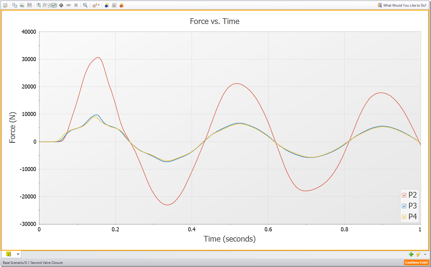
Note that at Time = 0 seconds, there are no forces for any of the force sets. This is expected since the sum of forces across a piping run between two elbows equals zero in a steady-state system. If a Point or Exit type force set were used instead of a Difference type force set, then a non-zero force may be encountered during the steady-state.
Additionally, some traditional methods of analyzing force sets will not yield the same results as AFT xStream since they may not include friction or momentum effects in their force balances. Traditional methods can yield significantly different results and indicate incorrect, non-zero forces during steady-state conditions.
There are two important points to be observed here:
-
AFT xStream calculates transient fluid forces. This does not include weight from piping, components, or the fluid itself, or any other forces external to the piping. A comprehensive analysis of pipe loading must separately include these items.
-
Ignoring friction and momentum force balance components will result in force imbalances that do not exist in reality.
Step 9. Run the other child scenarios
-
ØRun the other two child scenarios and load the Force Sets graph list item for each. The results are shown in the figures below.
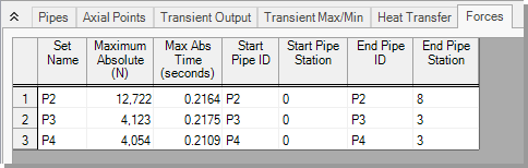
Figure 13: Forces tab in the Output window for the "0.25 Second Valve Closure" scenario
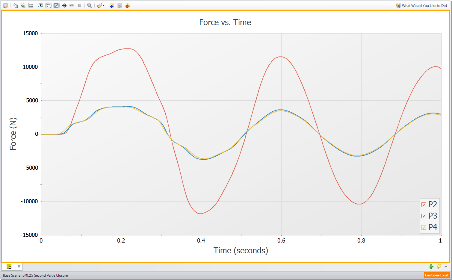
Figure 14: Force vs Time graph for the "0.25 Second Valve Closure" scenario
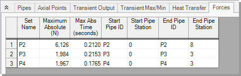
Figure 15: Forces tab in the Output window for the "0.5 Second Valve Closure" scenario
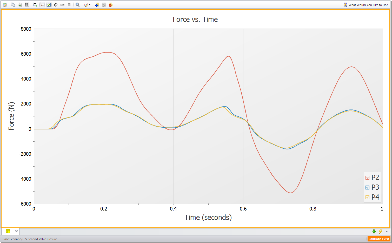
Figure 16: Force vs Time graph for the "0.5 Second Valve Closure" scenario
These figures show that the maximum force magnitude increases as the valve closes faster. Typically, the more rapidly a change occurs, the more severe the resulting forces are. Therefore, a utility of AFT xStream would be to evaluate the correlation between transient event duration (e.g., valve closing time) and the resultant force magnitudes.
Factors affecting the timing and magnitude of forces
The pipe sectioning, fluid property model, and specification of the Maximum Pipe Mach Number During Transient setting can have a significant effect on the accuracy of the forces calculated by AFT xStream. These effects are not significant for the system built within this example. However, the results for altering each of these three parameters are shown in the figures below so that you may see the impact of changing these three parameters. Note that in Figure 18, Steam from the ASME Steam, Chempak, and NIST REFPROP fluid libraries are superimposed on each other, indicating no meaningful difference for this case.
If you wish to learn more about the effect of altering these 3 factors with regards to force, see the Transient Sensitivity Analysis Tutorial.
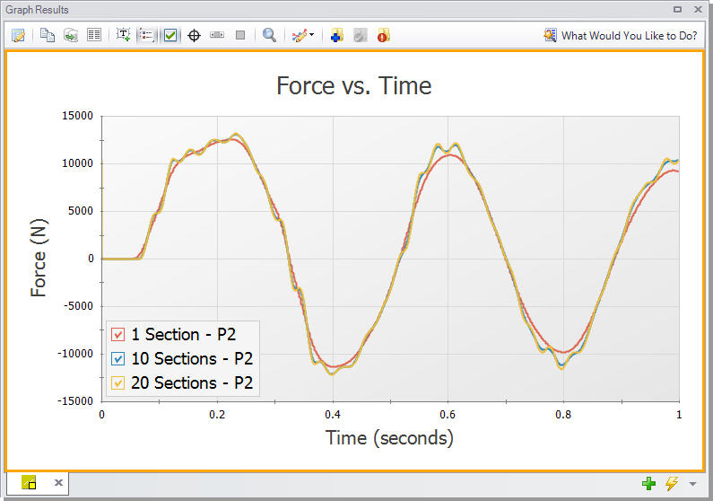
Figure 17: Effect of sectioning when all scenarios use the AFT Standard fluid library and a Maximum Pipe Mach Number During Transient of 1
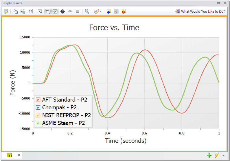
Figure 18: Effect of the fluid property model when all scenarios use a Minimum Number of Sections Per Pipe of 1 and an Estimated Maximum Pipe Mach Number During Transient of 1
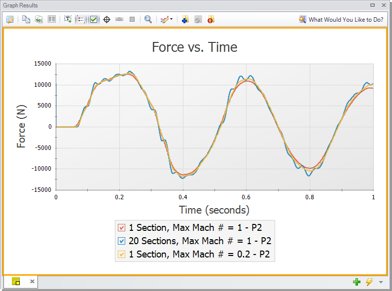
Figure 19: Effect of Maximum Pipe Mach Number During Transient when all scenarios use the AFT Standard fluid library
Step 10. Export to a CAESAR II Force File
-
ØOpen the Output window, and click on the File menu. Select Export Force File... and choose CAESAR II® Force File. This will open the export file window shown in Figure 20.
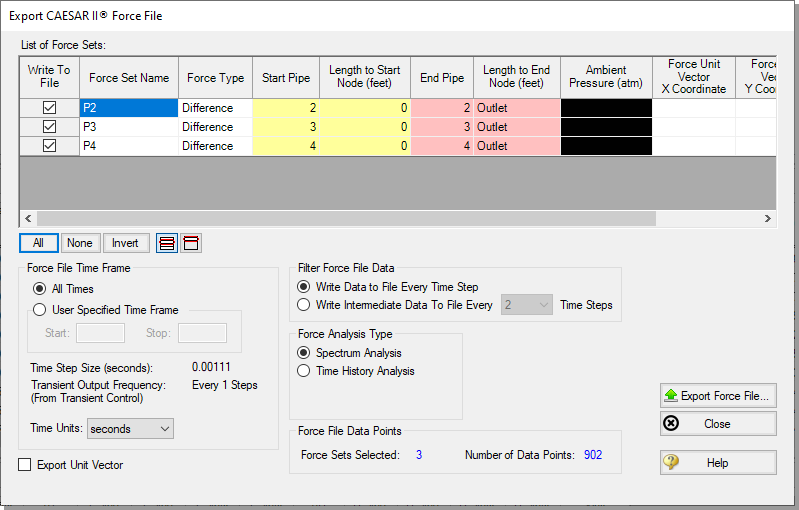
The force sets to include in the force file may be individually selected, along with how frequently data points are saved. The number of data points that will be in the file is also displayed for the given settings. This number should not exceed the maximum number of data points allowed for the relevant piping stress software, which in the case of CAESAR II® is 2500.
If unit vector information has been entered in the Force Definitions panel, the Export Unit Vector option can be used to include this information in the exported file. Similar methods to those described above can be used to export force files to ROHR2®, TRIFLEX®, and AutoPIPE®.
Conclusion
Force sets were defined to calculate the transient forces between pairs of 90 degree elbows (represented by lossless Branch junctions) as a result of two simultaneous Turbine Safety Valve closures in a steam system. Several child scenarios were created to evaluate the effect of the closure time where we noted that a faster valve closure produced higher magnitudes of forces. Several important assumptions and takeaways were discussed:
-
The Difference force type is intended to model the specific case where all of the following criteria is true:
-
The force is between a pair of 90 degree elbows
-
The force is an axial pipe force
-
All pipes, fittings, and components between the elbow pair are in-line
-
-
AFT xStream calculates transient fluid forces. This does not include weight from piping, components, or the fluid itself, or any other forces external to the piping. A comprehensive analysis of pipe loading must separately include these items.
-
Ignoring friction and momentum force balance components will result in force imbalances that do not exist in reality.
Finally, we discussed how to export these forces into a force file to be used in pipe stress analysis software.


