Curve Fitting
There are many places in AFT Arrow where the user is asked to define how a property changes in relation to another. Some examples are:
These properties are entered in a table format, relating one particular property to several others. For example, see the below definition of a custom fluid:
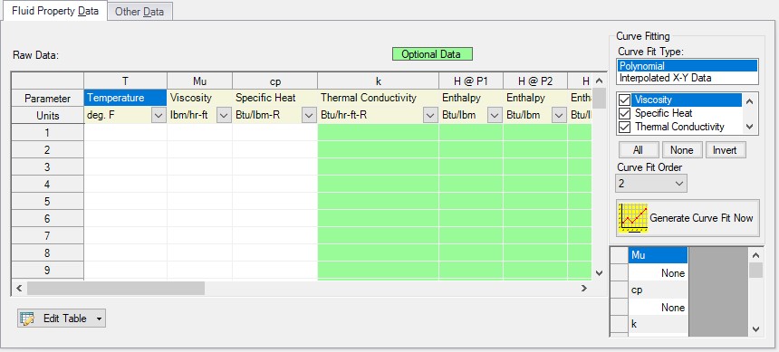
Figure 1: Custom Fluid Definition
There are several parameters that control the behavior of the fluid and they are entered as they relate to temperature.
However, it is important to recognize that these values in particular are not directly used in the solution. Instead, the data is used to create a best-fit curve. This curve is then used in the solution process. This is an important step to take because there must be a continuous relationship between the independent variable (e.g. temperature) and the dependent variable (e.g. density). Even if the final solution was close to one of the defined points, the solver needs continuous data to proceed.
There are some options for how the data is curve fit. First, there are two Curve Fit Types:
-
Polynomial - The data is best fit to a polynomial of order 0,1,2,3, or 4. Note that a 0th order polynomial is a constant value, and a 1st order is a linear fit.
-
Interpolated X-Y Data - The data has a linear interpolation drawn between every data point.
One of the critical items to note with any curve fit is that you may not be operating close to one of your defined points if the data does not conform well to a polynomial relationship. For example, the below fluid (a liquid) has a rapidly decaying viscosity that does not follow a polynomial relationship. Fitting the data to the standard 2nd order polynomial results in the following:

Figure 2: Using a Polynomial Curve Fit on Non-Polynomial Data
The viscosity relationship in the model will use the blue curve, and not the user-defined black points. Depending on the operating range of the system, this may significantly impact the results! For this data in particular, using the Interpolated X-Y Data option may be a better choice.
After data has been curve fit, the constants for the resulting curve are displayed in the lower right of the associated window.


