Air Distribution - ANS (English Units)
Air Distribution - ANS (Metric Units)
Summary
This example focuses on a closed loop cooling system that demonstrates some key features in using ANS to size a piping system. An existing model is used to investigate four potential sizing cases:
-
Size system for initial cost with a 5-year operating period
-
Size system for life cycle cost with a 5-year operating period
-
Size system for life cycle cost with an initial cost limit for a 5-year operating period
Note: This example can only be run if you have a license for the ANS module.
Topics Covered
-
Connecting and using existing engineering and cost libraries
-
Sizing for Initial or Life Cycle Cost and using Initial Cost Limits
-
Sizing a compressor and sizing piping for the chosen compressor
-
Interpreting Cost Reports
Required Knowledge
This example assumes the user has already worked through the Beginner: Air Heating System example, or has a level of knowledge consistent with that topic. You can also watch the AFT Arrow
In addition, it is assumed that the user has worked through the Beginner: Three Tank Steam System - ANS example, and is familiar with the basics of ANS analysis.
Model Files
This example uses the following files, which are installed in the Examples folder as part of the AFT Arrow installation:
-
Air Distribution.dat - engineering library
-
Air Distribution Costs.cst - cost library for Air Distribution.dat
-
Steel - ANSI Pipe Cost.cst - cost library for Steel - ANSI pipes
Step 1. Start AFT Arrow
From the Start Menu choose the AFT Arrow 9 folder and select AFT Arrow 9.
To ensure that your results are the same as those presented in this documentation, this example should be run using all default AFT Arrow settings, unless you are specifically instructed to do otherwise.
Open the US - Air Distribution - ANS Initial.aro example file listed above, which is located in the Examples folder in the AFT Arrow application folder. Save the file to a different folder.
Step 2. Define the Pipes and Junctions Group
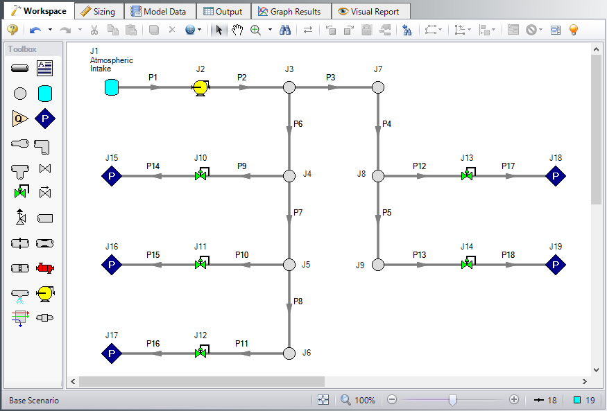
The Workspace should appear as shown in the figure below.
Overview of Sizing Systems with Compressors
A centrifugal compressor can be modeled with either the Compressor Curve or as a fixed flow rate or pressure/head as the Sizing option. Generally, if a specific compressor has been identified, the Compressor Curve type would be chosen, whereas the Sizing option is useful during the selection stage in order to identify the compressor requirements for the system. In some cases, even though the specific compressor has not been chosen, several candidate compressors are available. For this third case it would be best to model each candidate compressor with a compressor curve using separate scenarios for each compressor.
Sizing a Compressor
The compressor in our air distribution case is set as Sizing with a fixed flows of
As already stated, when a compressor is modeled as a fixed flow, it is not a specific compressor from a specific manufacturer. Thus, the costs for the compressor can only be approximated. To a first approximation, it should be possible to estimate the non-recurring cost (i.e., material and installation cost) for the pump as a function of power requirements. For instance, a typical ten horsepower compressor (of specific configuration and materials of construction for a given flowrate) may cost $2700, and a forty horsepower may cost $8250. Other typical costs for different power requirements can be approximated. The actual cost for the compressor will, of course, highly depend on the application. These costs are entered into a cost library and are accessed by the Solver. As AFT Arrow evaluates different combinations of pipe sizes, each combination will require a certain power from the compressor. With a cost assigned to this power, the ANS module can obtain a cost to enter into the objective which it sizes. Later in this chapter, we will look at the costs for the compressor in our example air distribution network.
In addition to non-recurring costs, recurring costs can also be estimated. Specifically, the cost of the power used by the compressor over a period of time (which the ANS module calls the System Life) can be determined. All AFT Arrow needs is an overall compressor efficiency to determine the actual power from the ideal power. Again, since we do not have a specific compressor selected yet, the efficiency can only be approximated. The ANS module calls this the Nominal Efficiency.
Therefore, it is recognized that at this first cut phase the values for nominal efficiency are imprecise and users may need to go through a few iterations to arrive at satisfactory results.
A step-by-step method of compressor selection proceeds in two phases. The steps are outlined in the Help System.
For this example, we will be completing the compressor selection process considering the objective of minimizing initial cost, then minimizing life cycle cost.
Step 3. Define the Automatic Sizing Group
The model is already defined for a regular AFT Arrow run, but we need to complete the sizing settings before running the analysis. Go to the Sizing window by clicking the Sizing tab.
A. Sizing Objective
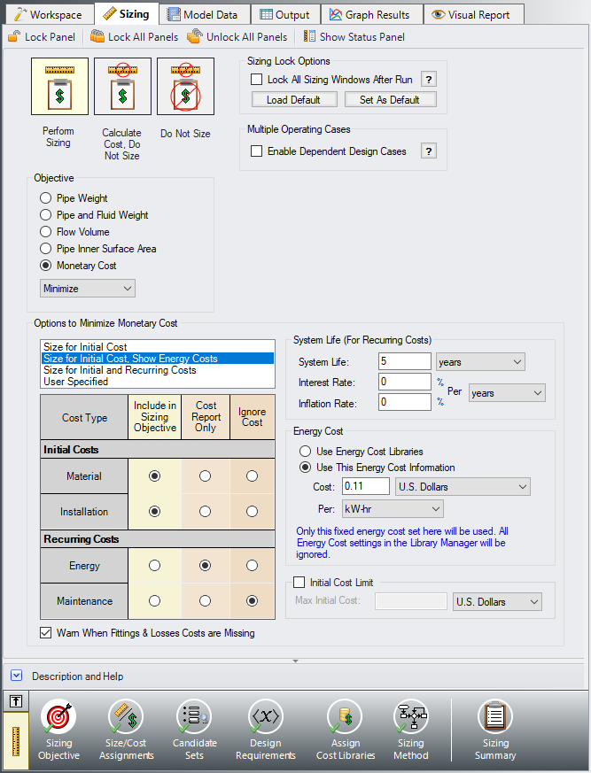
The Sizing Objective window should be selected by default from the Sizing Navigation panel along the bottom. For this analysis, we are interested in sizing the system considering the monetary cost for the initial costs only.
-
Select Perform Sizing for this calculation.
-
For the Objective, choose Monetary Cost and select the Minimize option from the drop-down list if these options are not already selected.
-
Under Options to Minimize Monetary Cost, choose Size for Initial Cost, Show Energy Costs. This will update the cost table to include both initial costs in the sizing calculation, and moves the Energy costs to be included in the Cost Report so that we can later compare the costs in this scenario to one where the Energy costs are included for the sizing. We do not have any information on Maintenance cost, so we will leave this cost in Ignore Cost.
-
Set the System Life to 5 years with 0% interest and inflation rates.
-
For the Energy Cost area choose Use this Energy Cost Information, with a cost of 0.11 U.S. Dollars Per kW-hr. Note this assumes the pump will run all day, every day, for the entire 5 years. Alternatively, we could have created an Energy Cost Library, which would be connected in the Assign Cost Libraries section. An Energy Cost Library allows variable energy costs to be used to account for varying prices during different times of day, different seasons, etc. For now, we are simplifying the input by using a fixed cost.
The Sizing Objective window should now appear as shown in Figure 2.
B. Size/Cost Assignments
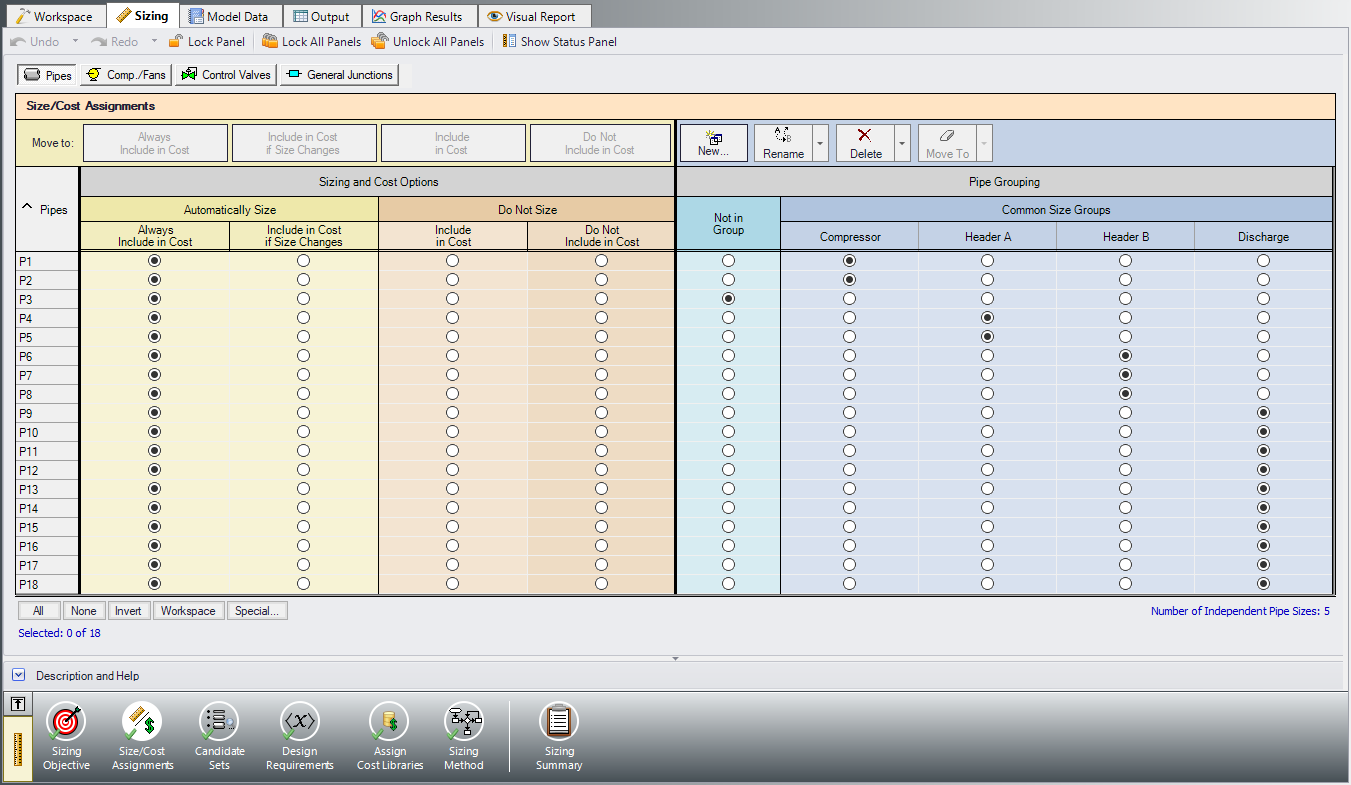
On the Sizing Navigation panel select the Size/Cost Assignments button. For this example we are sizing both the pipes and compressors for a new system, so we will need to calculate and minimize cost for all related components in the model.
ØClick All under the table to select all of the pipes, then click the Always Include in Cost button next to Move to. This will move all of the pipe selections to the corresponding column to be sized.
To decrease the run time and reduce complexity, as well as to enforce some design uniformity, it is useful to create Common Size Groups to link the pipes in different sections of the model.
For example, if all the 18 pipes are selected to be Not In Group, then 18 separate pipe sizes will be selected by the automatic sizing engine. That could potentially mean, for example, different pipe diameters in pipes P9 and P14. If one wanted pipes P9 and P14 to be sized to the same diameter, one would group them into a Common Size Group. To see how this works, in this model all discharge room piping will be put into a Common Size Group. What this means is that there will be a single diameter chosen for this group of pipes, rather than potentially six different diameters.
For this system we will define four groups to be sized in this model. To set the groups, it is standard to select pipes which must have the same size due to their placement relative to other pipes and junctions, such as pipes at the entrance and exit of valves. In Figure 3 we have identified these four groups.
First create a Compressor size group for pipes P1 and P2, which are highlighted in red.
ØClick New above the Pipe Grouping section to create the group, and name it Compressor. Select the radio buttons under the Compressor heading next to P1 and P2 to add them to the group. Alternatively, the pipes can be selected in the Workspace, then moved to a group by right-clicking the Workspace and selecting the corresponding option from the menu.
Repeat this process for the header piping. We will assume the header will have the same size, so therefore these pipes will have a common size. Like before, create a new group called Header A, and add the two header pipes on the right side of the system to the new group (pipes P4 and P5).
The headers supplying each room are one physical pipe in the field, represented as multiple pipes in AFT Arrow by necessity. Create two more groups and add the pipes as listed below and shown in Figure 4.
-
Header B = P6 - P8
-
Discharge = P9 - P18
The completed pipe Size/Cost Assignments can be seen in Figure 4. Note that pipe P3 should be the only pipe not in a group.
Note: Pipes in the Size/Cost Assignments table can be sorted by Common Size Group instead of sorting by number by clicking on the Pipe Grouping header. Clicking on the header for a particular group will sort the pipes in that specific group to the top of the window.
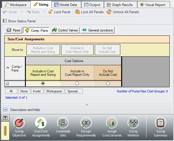
ØClick the Comp./Fans button to switch to the Compressor/Fan Size/Cost Assignments. Select the option to Include in Cost Report and Sizing for the compressor J2 as shown in Figure 5. The compressor will now be sized concurrently with the pipes.
Similar to the Common Size Groups for pipes, compressors can be placed into Maximum Cost Groups based on monetary cost. If compressor costs are added to a Maximum Cost Group, the ANS module will determine the compressor in the group with the maximum costs, and set all compressors in the group to use the largest cost. In this case there is only one compressor, so this option is not available.
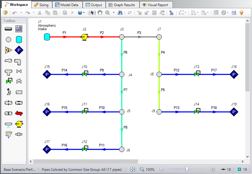
Now go to the Workspace window. It is possible to inspect the Common Size Groups in the model by coloring the pipes. From the View menu, select All under Color Size Groups. The model should appear as shown in Figure 3, though the colors may be different.
C. Candidate Sets
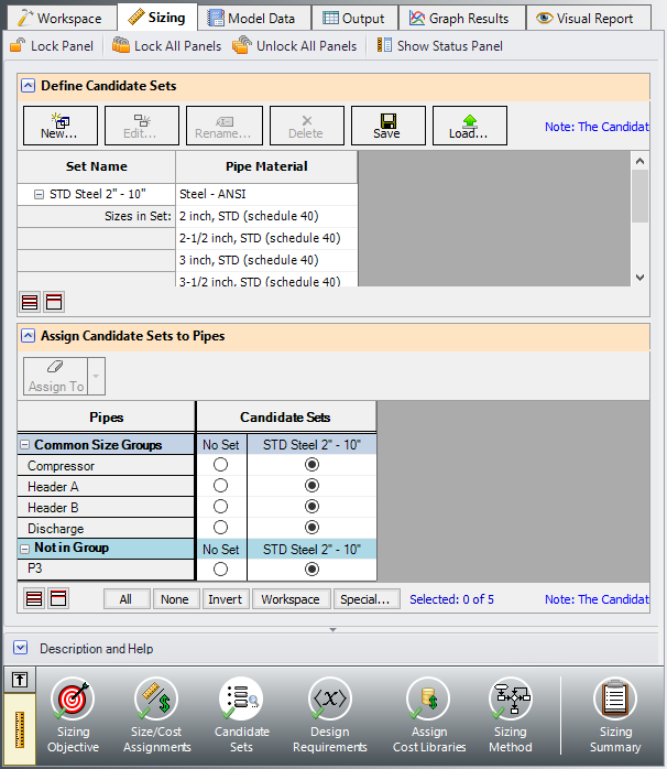
Click on the Candidate Sets button to open the Candidate Sets panel.
Create a new Candidate Set for all Steel - ANSI pipes between 2" and 10" in diameter. Click the New button, and name the Candidate Set STD Steel 2" - 10". Choose Steel - ANSI as the pipe material library, STD as the Material Type, and add all pipes from 2" to 10" in size.
In the bottom section of the window, check that each of the Common Size Groups and pipe P3 have been assigned to use the existing Candidate Set. The window should appear as shown in Figure 6.
D. Design Requirements
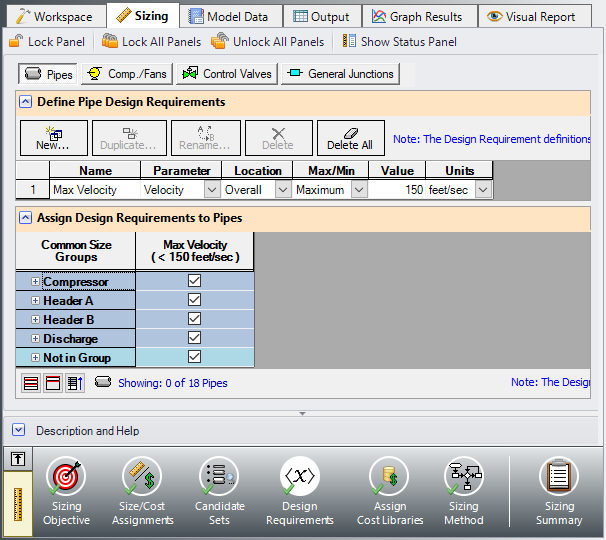
Select the Design Requirements button from the Navigation Panel.
For this model we have multiple requirements for the system:
-
All pipes have a maximum velocity of 150 feet/sec
-
All control valves must have a minimum pressure drop of 2 psid
-
All discharges must receive a minimum flow of 250 scfm
Define and assign the first requirement listed above as a Pipe Design Requirement as shown in Figure 7, and apply it to each of the pipes.
Notice that we have accounted for the minimum flow requirement in this system by using flow control valves in each discharge line. By using assigned flow compressor and flow control valves we have incorporated the necessary flow rate as a boundary condition, so we do not need to apply a Design Requirement to account for the second item.
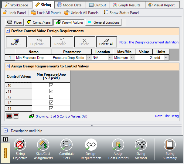
For flow control valves J10, J11, J13, and J14, define and apply the minimum pressure drop requirement in the Control Valves section as shown in Figure 8. Note that for compressor sizing purposes as discussed earlier control valve J12 has been defined as a Constant Pressure Drop valve, so the pressure drop Design Requirement does not need to be applied to this valve.
E. Assign Cost Libraries
Select the Assign Cost Libraries button. For this model the engineering and cost libraries have already been created, but we will need to connect and apply them.
Note: The Creating Libraries for Sizing a System example provides instructions on how to build the libraries for the first part of this example, and may be completed later for practice with creating libraries. The provided pre-built libraries will be needed to obtain the compressor curve data for Step 10 of this example.
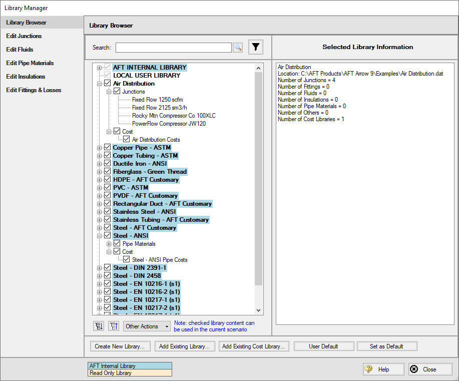
ØOpen the Library Manager by clicking the Library Manager button to see which libraries are connected. The AFT INTERNAL LIBRARY, LOCAL USER LIBRARY, and Pipe Material libraries should be available and connected by default. Available libraries will be shown based on libraries that Arrow has identified on your machine. The default connected libraries will be visible here, and additional libraries may be visible from other example files, or from libraries previously built and used on your machine.
This example uses one user-defined engineering library, Air Distribution.dat, which contains the data for the compressor. There are also two cost libraries, Air Distribution Costs.cst and Steel - ANSI Pipe Costs.cst, which contain the cost data for the junctions and the pipe materials, respectively. Air Distribution Costs.cst was built off of the engineering library Air Distribution.dat, and Steel - ANSI Pipe Costs.cst was built off of the Steel - ANSI Pipe Material library. To connect these libraries, do the following:
-
Click the button to Add Existing Library.
-
Browse to the AFT Arrow 9 Examples folder (located by default in C:\AFT Products\AFT Arrow 9\Examples\), and open the file titled Air Distribution.dat.
-
Repeat the above steps, but choose Add Existing Cost Library to browse for Air Distribution Costs.cst, then Steel - ANSI Pipe Costs.cst.
Note that it may be possible that the model file already has the cooling system libraries connected, in which case you will be notified that the library you are trying to add is already available. If the libraries are available, you will simply need to connect them by checking the box next to the library name for each of the three libraries.
Once these steps have been completed, you should now see that the new libraries have been added to the Available Libraries list, and have been automatically connected to the model, as shown in Figure 9 for the junction libraries. The junction libraries appear with the names Air Distribution, Air Distribution Costs, and Steel - ANSI Pipe Costs.
Note: When a library is selected in the Library Manager, the filename and location can be viewed in the Selected Library Information. Library names can be different from the given filename.
Once you have confirmed that the necessary libraries are connected, click Close to exit the Library Manager.
Since we are connecting a pre-built library, we will need to take an additional step to make sure that the compressor in the Workspace is linked to the Air Distribution engineering library that we added.
-
Go to the Workspace, and open the compressor (junction J2)
-
From the Library Jct list, select Fixed Flow
We have now re-connected the junctions that will be considered for the Cost Report and sizing calculations to the engineering library. This is important, since a junction must be connected to an engineering library before cost information can be assigned to it. Let's now return to the Sizing window.
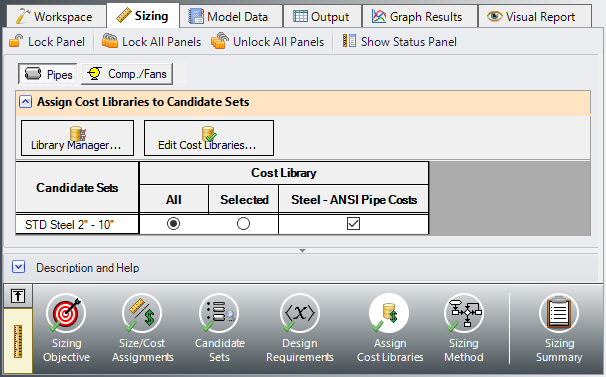
Back in the Assign Cost Libraries panel for the Pipes, the Steel - ANSI Pipe Costs library should be the only visible cost library, since it is the only connected library for the pipe sizes in the Candidate Set. Make sure that the library is checked to be applied for the model as shown in Figure 10.
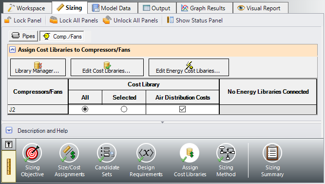
ØClick on the Comp./Fans button to view the cost library assignments for the compressor. The only visible library should be the Air Distribution Costs library, as this was the only cost library connected for the associated engineering library. Make sure that the checkboxes are selected under the library name so that the cost data will be applied for the compressor (Figure 11).
F. Sizing Method
Select the Sizing Method button to go to the Sizing Method panel.
Ø Choose Discrete Sizing, if not already selected, since it is desired to select discrete sizes for each of the pipes in the model.
For this model we have five independent pipe sizes as noted on the Size/Cost Assignments panel (four groups and pipe P3), and two design requirements (one pipe design requirement applied to all of the pipes, and a minimum pressure drop applied to four control valves). Due to the small number of independent sizes, it would be recommended to try the MMFD or SQP search method. Though it is not shown here, if both methods are run for this scenario the same solution will be obtained, though the Sequential Quadratic Programming (SQP) Method is slightly faster.
ØSelect Sequential Quadratic Programming (SQP) for the sizing method.
G. Sizing Summary
From the Sizing Navigation Panel select the Sizing Summary button.
The Sizing Summary panel allows the user to view all of the sizing input for the model in a tree view layout, which is shown in Figure 12. Items can be organized by sizing parameters (Design Requirements, Candidate Sets, etc.), or information can be viewed based off an individual pipe. For clarity these categories can be shown/hidden using the check boxes at the top of the panel.
Each tree node can be expanded/collapsed individually by using the ‘+’ and ‘-‘ buttons on the node. Alternatively, the buttons on the bottom of the panel can be used to collapse/expand all items. Right-clicking on the nodes provides additional options to collapse/expand items, view related nodes, or to copy information to the clipboard. The Sizing Summary panel can be printed from the printer button at the bottom of the panel.
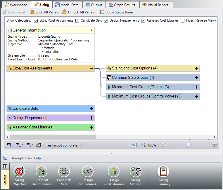
Figure 12: Sizing Summary panel layout with the Size/Cost Assignments expanded. The number of children nodes for each item can be seen in parentheses.
Step 4. Run the Model
Click Run Model on the toolbar or from the Analysis menu. This will open the Solution Progress window. This window allows you to watch as the AFT Arrow solver converges on the answer. Once the solver has converged, view the results by clicking the Output button at the bottom of the Solution Progress window.
Step 5. Examine the Output
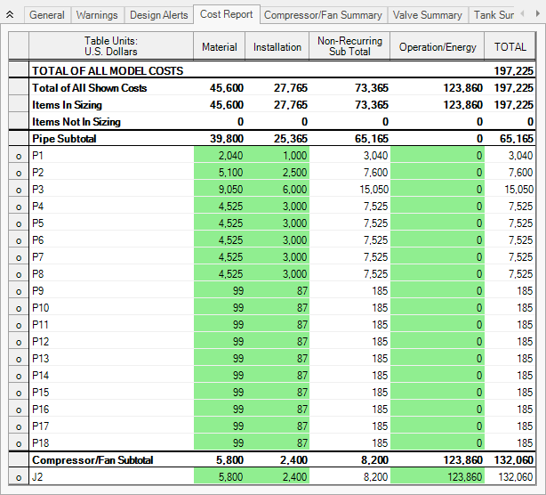
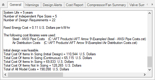
The Cost Report is shown in the General Section of the Output window (see Figure 13). The ANS module shows all costs in the Cost Report, including those that were not used in the automated sizing. The total cost for this system is
Other costs that are displayed in the Cost Report are Items Not in Sizing. These are items that have costs associated with them, but were not included in the automated sizing.
Note that the Items Not in Sizing total to
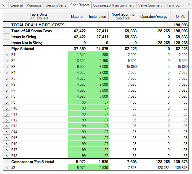
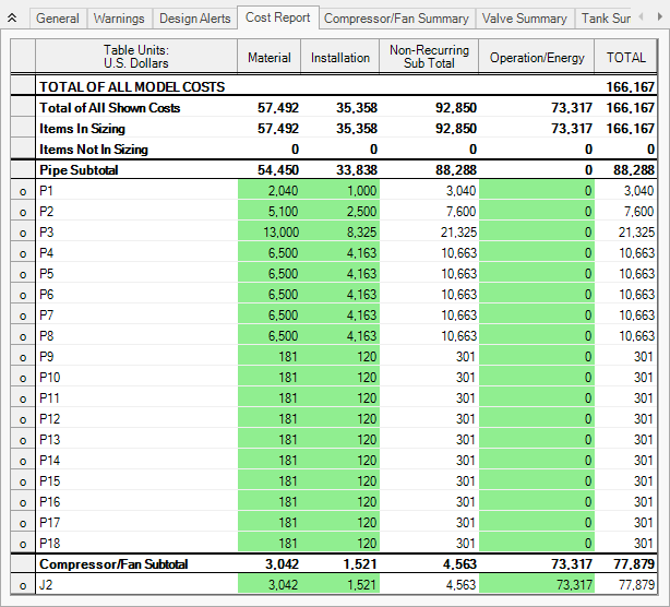
Figure 13: The Cost Report in the Output window shows the total and individual costs (in thousands of U.S. Dollars) for the sized system
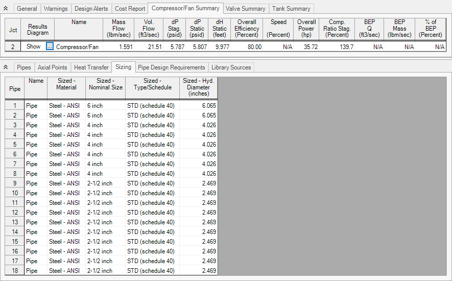
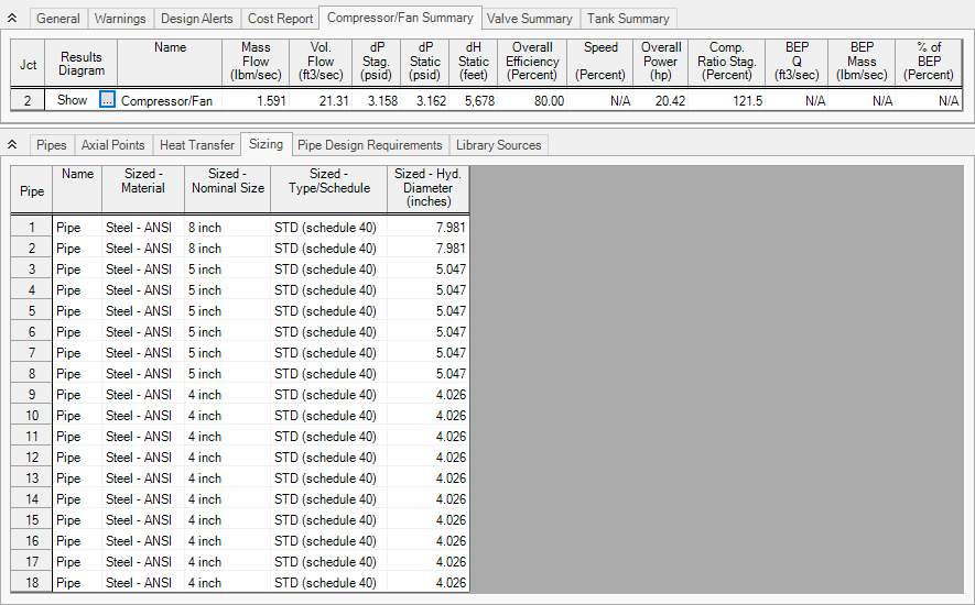
In the Pipes section of the Output window the final pipe sizes from the automated sizing can be seen, along with the Design Requirements status. For this model, the final system used pipe sizes varying from 2-1/2 to 6 inches, as seen in Figure 14. The information for the compressors can be seen in the Compressor/Fan Summary tab in the General Section, which is also shown in Figure 14.
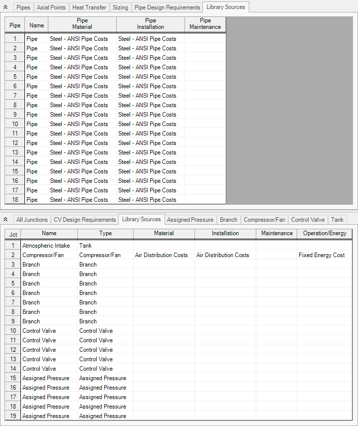
When a monetary cost objective is selected, additional tabs are available that display the Library Sources used for the Cost Report for each of the pipes/junctions. In this case both the Pipe Material and Pipe Installation costs for all of the pipes came from the Steel - ANSI Pipe Costs library which was connected earlier. Information for the compressor came from the Air Distribution Costs library. If multiple cost libraries are used for a category they will all be listed separated by commas. The Library Sources for the Pipes can be seen in Figure 15.
On the General tab of the Output window at the bottom of the report, the initial cost of the items included in the sizing can be seen, which was
Though not shown here, if the model is run using the objective to Calculate Costs, Do Not Size, it can be seen that the total cost for the system before sizing was
Step 6. Size the System for Life Cycle Cost over Five Years
From the Scenario Manager in the Quick Access Panel, we will create two children scenarios. With the base scenario selected, right click and choose Create Child. Name the new scenario Initial Cost. This scenario will store the initial cost sizing results we just obtained. Repeat this process to create a second child scenario, and name it Life Cycle Cost. For this scenario the only change that will need to be made is to update the Sizing Objective.
Go to the Sizing window, and make sure that the Sizing Objective button is selected. Under Options to Minimize Monetary Cost, choose Size for Initial and Recurring Costs. This will move the Energy costs selection to Include in Sizing Objective. The scenario is now complete.
ØClick Run from the Analysis menu to run the automated sizing. When the calculations have finished, click Output to view the results.
Step 7. Examine the Output
After viewing the Cost Report, it can be seen that the overall cost is now
Taken on its own, this new cost represents a savings of about $32,000 over the Initial cost scenario which was sized based on Initial Cost only. This represents a 14% cost reduction. In the initial cost scenario, the non-recurring cost was $69,833, while the overall cost was $198,098. Now the non-recurring cost is $92,850 while the overall cost is $166,167. The initial cost thus increased by about $23,000 in order to reduce the operating cost from $128,265 to $73,317 (a reduction of about $55,000). The source of the operating cost is the cost of power for the compressors. To reduce compressor power usage, it makes sense to increase the pipe size and thus reduce frictional losses. The larger pipe sizes can be reviewed by looking at the Sizing tab in the Pipe Output section, as shown in Figure 18.
Considering this cost breakdown between the scenarios highlights the importance of choosing to include the energy costs in the initial cost scenario. If they were not in the Cost Report of the initial cost scenario, the total cost would be
By performing both analyses the designer has quantitative data on the impact of initial cost design on operational costs of the system, and can make an informed design choice.
Step 8. Size the System for Life Cycle Cost with Initial Cost Limit
While the energy cost savings from life cycle cost sizing are desirable, the budget for the project may not support the higher initial cost that is required. In that case, we can apply an initial cost limit to the life cycle cost sizing.
Clone the Life Cycle Cost scenario. Name the scenario Initial Cost Limit.
ØReturn to the Sizing Objective panel and select the option for Initial Cost Limit. We will set the limit as $82,500 which is approximately an initial cost reduction of 25% from the original (un-sized) design. Run the model and go to the Output tab.
A summary of the results with the initial cost limit compared to each of the initial and life cycle cost sizing scenarios for a five year life cycle can be seen in Table 1. Notice that while the material and installation costs were similar to the costs from the initial cost scenario, the energy costs were decreased by about $10,000. These energy costs were achieved by increasing the compressor pipe sizes, while decreasing the header pipe sizes to achieve a better efficiency in the compressor. Table 2 shows a comparison of the pipe sizes throughout the system for the original design, and each of the sizing scenarios.
Table 1: Cost Summary of Sizing Runs for the Air Distribution System
| Scenario | Material | Installation | Non-Recurring Sub Total | Energy | Total | Reduction |
|---|---|---|---|---|---|---|
| Not Sized | 67,456 | 43,088 | 110,544 | 68,083 | 178,626 |
|
| Initial Cost | 42,422 | 27,411 | 69,833 | 128,265 | 198,098 | -20,000 |
| Life Cycle Cost | 57,492 | 35,358 | 92,850 | 73,317 | 166,167 | 12,600 |
| Initial Cost Limit | 45,138 | 27,971 | 73,109 | 117,888 | 190,997 | -12,200 |
Table 2: Summary of final pipe sizes for Common Size Groups in the Air Distribution System
| Scenario | Compressor | Header A | Header B | Discharge | Pipe P3 |
|---|---|---|---|---|---|
| Not Sized | 6 inch | 6 inch | 6 inch | 3 inch | 6 inch |
| Initial Cost | 6 inch | 4 inch | 4 inch | 2-1/2 inch | 4 inch |
| Life Cycle Cost | 8 inch | 5 inch | 5 inch | 4 inch | 5 inch |
| Initial Cost Limit | 8 inch | 4 inch | 4 inch | 3-1/2 inch | 4 inch |
Step 9. Automated Sizing with Compressor Curve Data
As discussed in the previous section summarizing the compressor selection process, once the compressor is sized then actual compressors can be modeled. The actual compressor should closely match the sizing results in the following areas: generated pressure at the design flow, efficiency at the design flow, and cost. Let's apply actual compressor data for the case that was sized for life cycle cost with an initial cost limit to complete phase two of the compressor selection process above.
Reviewing the results for the life cycle cost with initial cost limit scenario one can see that the sized system calls for a compressor of about
Based on the sizing analysis, we will choose a compressor from the (fictitious) Rocky Mountain Compressor Company. Its model 100XLC is a close match for the requirements of a 5-year life cycle design. The model 100XLC has the following characteristics: at 1250 scfm its pressure is 5.6 psid and efficiency is 80%. Its material cost is $5,800 and installation cost is $2,400. To setup a new scenario for the system with the candidate compressor data:
In the Scenario Manager clone the Initial Cost Limit child scenario and name it Actual Compressor Curve.
In the new scenario, open the properties window for compressor J2 select
In the Flow Control Valve Property window for J12, change the Valve Type to Flow Control (FCV), and enter a Flow Setpoint of
Go to the Sizing window, then navigate to the Design Requirements panel. Select the Control Valves button at the top of the window.
Apply the Min Pressure Drop design requirement to Control Valve J12.
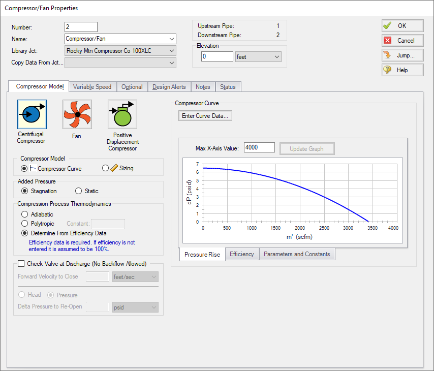
Figure 19: Compressor Properties window with the Rocky Mtn Compressor Co 100XLC library item selected
The necessary changes are now complete to size the system with the updated compressor and flow control valve data.
ØSelect Run from the Analysis menu to perform the automated sizing. When the solver has finished, click Output to review the results, as can be seen in Figure 20.
The Cost Report shows a total sized cost of
Now we have sized the system for use with an actual compressor.