Review of Compressible Flow Theory
This topic gives an overview of internal compressible flow theory. For a more complete development of compressible flow theory, please consult one of the many textbooks available
What is Compressible Flow?
Compressible flow is a specialized branch of fluid mechanics that describes the flow of gases. This field of study is sometimes called gas dynamics.
Compressible flow theory draws heavily from the fields of fluid mechanics and thermodynamics. This important branch of fluid mechanics has been developed almost completely since the year 1900. Its development has been largely driven by the extraordinary progress in the applied fields of aerodynamics and aircraft technology.
The field of compressible flow breaks down naturally into the two related areas of internal and external flow. Among the important applications of external compressible flow are the design of aircraft and airfoil design. Among the important applications of internal compressible flow are pipe flow, nozzles and gas turbines. In AFT Arrow, the interest is entirely in internal compressible flow.
The basic feature that distinguishes compressible from incompressible flow is the changing density of the gas. The density of the gas is related to the temperature and pressure of the gas through an equation of state. The variable density makes traditional incompressible analysis techniques of limited usefulness, and in general makes pipe flow analysis much more complicated.
The variable gas density has several important ramifications. First, the velocity of the gas is related to density through the continuity equation, and thus velocity also becomes a variable even in constant area pipes. Second, the density dependence on temperature means that the energy equation is coupled to the equation of state and must be solved simultaneously with the other governing equations. And last, the velocity of the gas is constrained by the sonic gas speed. Thus, unusual effects like sonic choking can occur, which further complicates analysis.
It should be noted that not all gas flows see significant compressible flow behavior. In some applications the gas velocities are low enough or the pressure drops are small enough that compressible effects are insignificant. In such situations, systems can be modeled with traditional incompressible techniques. AFT Arrow is capable of modeling any gas flows.
Equation of State
The equation of state relates the density, pressure and temperature of a gas. In principle, knowledge of any two of these parameters makes it possible to determine the third.
The Ideal Gas equation of state is given by the following

where
![]() is the universal gas constant and
is the universal gas constant and
![]() is the molecular weight of the gas. These two terms are frequently combined into a constant Rg
is the molecular weight of the gas. These two terms are frequently combined into a constant Rg
|
|
(63) |

where Rg is the gas constant for the particular gas. The above equation is known as the ideal gas equation, because it offers an idealized model to relate the pressure, density and temperature of a gas. For simplicity, the g subscript will be dropped and it is to be understood that R is not the universal constant, but that for a particular gas.
Experiments have shown that Equation 63 can be applied to a more general selection of gases by introducing the compressibility factor, Z, which compensates for departure from ideal gas behavior.
|
|
(64) |

There are many methods of determining Z. These methods are found in textbooks and handbooks, each having strengths and weaknesses.
First Law and Isentropic Relationships
From the First Law of Thermodynamics we know that
|
|
(65) |

For a reversible process, the work term can be represented by the following
|
|
(66) |

where v is the gas specific volume (inverse of density). In addition, the incremental addition of heat is given by
|
|
(67) |

where s is the entropy. Substituting Equations 66 and 67 into 65 and rearranging yields
|
|
(68) |

The enthalpy is related to the internal energy by the following identity
|
|
(69) |

Differentiating yields

so that Equation 68 becomes
|
|
(70) |

By using a suitably average specific heat constant, the enthalpy can be related to temperature
|
|
(71) |

and can be substituted into Equation 70 to obtain

The specific volume is the inverse of density, thus
|
|
(72) |

To simplify the following concepts, a perfect gas will be assumed and extensions to real gases will be made without proof. Later applications will describe the effects of real gas behavior in more detail.
For a perfect gas, the third term in Equation 72 can be modified to obtain
|
|
(73) |

Integrating Equation 73 results in
|
|
(74) |

In many applications the local gas flow is isentropic, which causes the left side of Equation 74 to go to zero yielding
|
|
(75) |

For an ideal gas it can be shown that
|
|
(76) |

or rearranging
|
|
(77) |

where γ is the ratio of specific heats.
For a real gas, Equations 76 and 77 become
|
|
(78) |

|
|
(79) |

The ratio of specific heats can also be calculated by
|
|
(80) |

The parameter γ is very important in determining the thermodynamics in isentropic processes. When considering a real gas, as the pressure increases Equation 80 takes on a modified form (BejanBejan, A., Advanced Engineering Thermodynamics, John Wiley & Sons, New York, NY, 1988., 1988, pp. 178)
|
|
(81) |

By algebra Equation 75 becomes
|
|
(82) |

By similar methods it can be shown that
|
|
(83) |

To summarize, Equations 82 and 83 are isentropic relationships that are valid for real gases if the appropriate value for γ is used.
The sonic speed of a gas is the velocity at which disturbances propagate within a gas. Unless a system is specially designed to produce supersonic flow, the sonic flow speed is the maximum speed at which the gas can travel.
It can be shown that a sound wave is an isentropic phenomenon involving virtually no energy loss, and that the speed of sound is given by the following equation (based on mass and momentum conservation)
|
|
(84) |

where a is the speed of sound and the subscript “s” refers to isentropic conditions. Another more useful form of Equation 84 is obtained by combining Equations 82 and 83 to relate pressure and density
|
|
(85) |

Using Equation 85 in Equation 84 and carrying through the differentiation

or using the ideal gas equation (Equation 63)
|
|
(86) |

Equation 86 is the classic equation for speed of sound, and since the specific heat ratio varies only slightly, the speed of sound effectively depends only on temperature.
For real gases, Equation 86 requires using the real gas equation (Equation 64) to obtain
|
|
(87) |

As an example of sonic velocity, consider air at 70º F (530º R). The specific heat ratio for air is about 1.4, and assuming ideal gas (Z = 1) then

The relationship between the gas velocity and sonic speed is known as the Mach number.
|
|
(88) |

The Mach number is a dimensionless quantity that is the most important parameter in compressible fluid flow. Relating all parameters to the Mach number greatly simplifies compressible flow calculations.
In general, the sonic gas velocity is the maximum that can be attained in a system, thus the largest Mach number in a pipe system is 1. This is known as sonic flow. Flows less than Mach 1 are referred to as subsonic flows. It is in fact possible to attain Mach numbers greater than 1 by using a specially designed convergent-divergent nozzle. Flows greater than Mach 1 are referred to as supersonic flows. There are special applications for supersonic flows in internal flow systems, however these applications are not generally of interest to the piping engineer and thus no attempt is made to address supersonic flows in AFT Arrow. AFT Arrow strictly assumes that Mach 1 is the maximum in the system.
Stagnation Properties in Compressible Flow
In application of Equation 65 to compressible pipe flow, use of the fluid enthalpy simplifies energy balance calculations. The enthalpy is a convenient parameter that combines the internal energy changes with the work performed by volume changes in the flow. The energy equation is:
|
|
(89) |

A new parameter called the stagnation enthalpy is introduced which is defined as:
|
|
(90) |

Introducing Equation 71 into Equation 90 results in
|
|
(91) |

where To is the stagnation temperature. The stagnation properties are sometimes referred to as "total" properties. In contrast, the temperature, T is the thermodynamic temperature that we are accustomed to, and takes on the more descriptive name of static temperature.
Using Equation 79 to replace cp results in
|
|
(92) |

and using the Mach number, Equation 88, this becomes
|
|
(93) |

Equation 93 relates the stagnation and static temperatures through the single flow parameter Mach number and γ, which is frequently constant.
Following from Equation 82 and 83
|
|
(94) |

|
|
(95) |

Between pressure, temperature, enthalpy and density, it is easiest to grasp the physical difference between static and stagnation properties when considering pressure. The classic example is a pitot tube that is normal to the flow or pointed directly into the flow. Figure 1 depicts the distinction.
The ratio of stagnation to static conditions for pressure and temperature are shown in Figure 2.
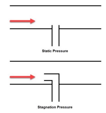
Figure 1: Comparison of static and stagnation pressure measurement at a pitot tube
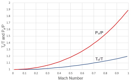
Figure 2: Variation of stagnation to static temperature ratio and stagnation to static pressure ratio with Mach number. Gamma = 1.4.
The stagnation temperature, stagnation enthalpy and stagnation pressure (and to a lesser extent, stagnation density) are of great importance in compressible flow systems. The stagnation property is made up of the “static” portion (which is the thermodynamic portion) and the “dynamic” portion (due to the fluid motion). The stagnation property is that property that would exist if the flow was brought to rest. In a fluid at rest (such as a large tank) the stagnation and static properties are equal.
The stagnation properties take on significance because they combine the effect of fluid velocity. Thus, a frictionless pipe will have constant stagnation pressures even if the area (and hence velocity) changes. The stagnation enthalpy will remain constant as long as no heat transfer and no elevation change occurs (see Equation 89). If the stagnation enthalpy is constant, the stagnation temperature remains constant insofar as Equation 71 remains valid. Departures from Equation 71 mean that the stagnation temperature can change in an adiabatic pipe, but this change is usually small. For a perfect gas, Equation 71 is always valid and thus stagnation temperature is always constant in adiabatic flow.
The convenience of stagnation properties is that frictional pressure loss and heat transfer calculations can be performed by using the stagnation property, thus avoiding the need to separately calculate dynamic (velocity) effects.
Also of importance is the issue of pipe networks. When a branch exists in a compressible flow network, a change in flow area is almost certain. The change in flow area means a change in velocity, and hence a change in the static pressure and static temperature. However, the stagnation pressure and temperature must always match at branching boundaries. The result is that the stagnation pressure and temperature are the key variables to solve for in a network pipe system.
The Continuity Equation
The continuity equation is the equation that applies the Law of Mass Conservation. For steady flow, the vector integral form of the continuity equation is given by
|
|
(96) |

Carrying out the integration of Equation 96 and assuming one-dimensional flow in a pipe results in
|
|
(97) |

If the pipe is of constant area, Equation 97 can be differentiated to obtain the following
|
|
(98) |

Equation 98 states that any increase in gas density must be accompanied by a decrease in velocity.
The Momentum Equation
The momentum equation is an expression of Newton’s Second Law of Motion, which states that the change in momentum is proportional to the sum of the acting forces, or
|
|
(99) |

For gas flow in a pipe, the acting forces are the pressure forces and friction forces. Assuming one-dimensional flow in a constant area pipe, the differential form of Equation 99 is
|
|
(100) |

where τw is the wall shear stress. The wall shear stress can be expressed in terms of a Moody friction factor, f (one-fourth of the sometimes used Fanning friction factor), and defined as
|
|
(101) |

Substituting Equation 101 into Equation 100 results in
|
|
(102) |

Equation 102 relates the change in fluid momentum (the third term) to the pressure forces (first term), friction forces (second term) and body forces (fourth term). The four terms balance to zero.
The Energy Equation
The First Law of Thermodynamics was introduced earlier in Equation 89,
|
|
(89) |

or, using the stagnation enthalpy (Equation 90), the energy equation becomes
|
|
(103) |

In the case of constant elevation, dz is zero and Equation 103 states that any heat transfer in a pipe is accompanied by a proportional change in stagnation enthalpy. If no heat transfer occurs (adiabatic flow), the stagnation enthalpy is constant.
For a perfect gas, the enthalpy is related to temperature by Equation 71. In general, enthalpy is a function of static temperature and pressure

While it is tempting to relate stagnation conditions on a similar basis because of the simplifications that result, in general only static conditions should be used. Thus

Frictional Effects in Pipes
To clearly understand the effect of friction in a pipe, it is convenient to look at the case of isothermal flow. The momentum equation, Equation 102, will be used as the starting point. Neglecting gravity effects,

From the continuity equation (98)

Substituting this into the momentum equation

For ideal gas, isothermal flow,
|
|
(104) |

Therefore

or using the Mach number

or
|
|
(105) |

For subsonic flow, the quantity on the right hand side will always be negative. Therefore, dP will always be negative when there is isothermal flow with friction, which is what one would expect. If dP is negative

then from the equation of state (104)

Therefore, from the continuity equation (98)

The conclusion therefore is that in isothermal frictional pipe flow, the velocity will always increase along the pipe. Simply put, the gas will accelerate. It can also be shown that the gas will accelerate if the flow is adiabatic. This further means that the Mach number will increase along the pipe length, eventually reaching Mach 1 sonic conditions if the pipe is long enough.
Once sonic conditions are reached, no additional acceleration is possible. Thus the flow will experience sonic choking. When a flow experiences sonic choking, lowering the downstream pressure to increase the differential pressure will not increase the flow. This phenomenon is frequently encountered in long gas transfer lines, and is addressed by placing compressors in the pipeline at regular intervals.
It should be noted for completeness that the previous development assumed isothermal flow.
If pipe conditions are such that a gas is cooled along its length, then it is possible to decelerate a compressible flow. The reason decelerating flow can occur when the gas is cooled is seen from the equation of state. The ideal gas equation, in differential form, is

and eliminating density using the continuity equation

If cooling occurs, then the temperature change is negative, and because the pressure change is also negative, the velocity change can be either negative or positive. Thus, accelerating or decelerating flow is possible. In most applications, the pressure changes more rapidly than the temperature, making the velocity change positive resulting in accelerating flow.
Isothermal and Adiabatic Flow
Since the majority of gas flow applications operate somewhere between isothermal and adiabatic flow, these two idealized cases are frequently taken as the extremes to consider. As discussed in the previous section, this is not strictly true.
The case of adiabatic flow is frequently encountered in short pipelines or in cases where the pipes are well insulated. When the flow is adiabatic, the static temperature will decrease along the pipe. This can be seen from Equation 93. For perfect gases, the stagnation temperature is constant in adiabatic flow. As the Mach number, M, increases, the static temperature must decrease.
But what happens when the pipe is cooled? When cooled, the stagnation temperature will decrease and the static temperature will actually decrease more than it would naturally. Thus, we can see that adiabatic flow cannot always be relied upon to be an extreme case.
The case of isothermal flow is frequently encountered in long gas transfer pipelines. When the flow is isothermal, then by definition the temperature remains constant. This can only occur if the gas is heated from its tendency to cool down. In a long transfer line exposed to ambient conditions, the tendency is for the gas pipe material to come to equilibrium with the surroundings, and the gas will tend toward equilibrium with the ambient conditions as well. The gas is heated by the ambient conditions outside the pipe.
In a more general case of gas heating, the heating may be strong enough to actually increase the static temperature. This means that the isothermal condition is not the extreme limit either. There is, in fact, no limit to gas heating effects until conditions reach ionization or dissociation.
Figure 3 shows an example of air flow in a pipe where the adiabatic and isothermal flow do not bracket the range of possible flow conditions.
This discussion points out a frequent misconception among engineers that isothermal and adiabatic flow are the extreme cases to consider in gas flows. A more accurate statement is that the conditions under which the majority of gas pipelines operate have heat transfer boundary conditions that maintain the gas between adiabatic and isothermal behavior. For most practical applications, adiabatic and isothermal flow can be considered as the extreme cases. But it has been shown that this is not a completely general rule, and may be incorrect in some applications.
One last comment of practical importance. Whether a pipe operates adiabatically or isothermally or somewhere in between or outside, the primary impact of these assumptions is on the gas temperature.
Frequently, for analysis simplification purposes, a gas is assumed to operate either adiabatically or isothermally, and the result is that the flow rates and gas pressures in the system do not change significantly between these two idealized cases. Thus, if the purpose of the analysis is to determine the system flow rate or flow distribution in a network, the heat transfer assumption used for the pipe will frequently have only a second order effect on the results.
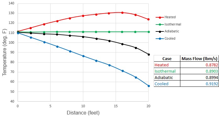
Figure 3: Comparison of temperature profiles and flow rate predictions for adiabatic, isothermal, heated and cooled air flow in a 20 ft. long 1 inch steel pipe. Inlet conditions are 100 psia, 111 °F and outlet pressure is 60 psia. Cooled flow has ambient temperature of 30 °F. Heated flow has ambient temperature of 220 °F. Both heated and cooled cases have pipe wall and insulation heat transfer coefficients which total to 100 Btu/hr-ft2-F. Note how adiabatic and isothermal cases do not bracket conditions. See Walters (2000)Walters, T.W., "Gas-Flow Calculations: Don't Choke", Chemical Engineering, Chemical Week Associates, Jan. 2000, pp. 70-76..


