Beginner: Three Reservoir Problem - ANS (English Units)
Beginner: Three Reservoir Problem - ANS (Metric Units)
Summary
The objective of this example is to familiarize the user with the panels in the ANS module. We will apply automated sizing to determine the ideal pipe sizes from our previously built three-reservoir model to reduce costs while meeting certain requirements.
Note: This example can only be run if you have a license for the ANS module.
Topics Covered
-
Minimizing the flow volume to minimize cost
-
Specifying Pipe Design Requirements
-
Choosing Candidate Sets
Required Knowledge
This example assumes the user has already worked through the Walk-Through Examples section, and has a level of knowledge consistent with the topics covered there. If this is not the case, please review the Walk-Through Examples, beginning with the Beginner: Three Reservoir Model example. You can also watch the AFT Fathom Quick Start Video Tutorial Series on the AFT website, as it covers the majority of the topics discussed in the Three-Reservoir Model example.
Model Files
This example uses the following files, which are installed in the Examples folder as part of the AFT Fathom installation:
Step 1. Start AFT Fathom
From the Start Menu choose the AFT Fathom 12 folder and select AFT Fathom 12.
To ensure that your results are the same as those presented in this documentation, this example should be run using all default AFT Fathom settings, unless you are specifically instructed to do otherwise.
Step 2. Open the model
Open the
We will be using the Base Scenario to compare the original results without Sizing to the results with Sizing. Create a child scenario named Sized.
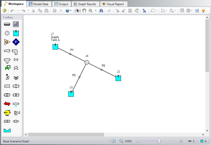
The workspace should look like Figure 1 below:
Step 3. Define the Modules Panel
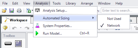
Open Analysis Setup from the toolbar or from the Analysis menu. Navigate to the Modules panel. For this example, check the box next to Activate ANS and select Network to enable the ANS module for use. A new group will appear in Analysis Setup titled Automatic Sizing. Click OK to save the changes and exit Analysis Setup. A new Primary Window tab will appear between Workspace and Model Data titled Sizing. Open the Analysis menu to see the new option called Automatic Sizing. From here you can quickly toggle between Not Used mode (normal AFT Fathom) and Network (ANS mode).
Figure 2 below shows the Analysis menu options when ANS is activated.
Step 4. Configure Sizing Settings
Here we will pursue a brief introduction to some of the sizing capabilities in the ANS module. A more complete discussion is given in the AFT Fathom Help file.
The Sizing window is comprised of multiple panels which can be accessed using the buttons on the Sizing Navigation panel along the bottom of the window, as shown in Figure 3. The sizing panels can be accessed in any order, though it is easiest to enter the information by navigating the panels from left to right, since the input on panels such as the Sizing Objective and Sizing Assignments panels will affect the options available on later panels. Depending on the type of sizing being done, some panels may be disabled or unused.
Each panel button contains either a green checkmark or red circle which denotes the completion status of that panel. If the minimum required information is present to run the model, the symbol will be green, whereas the red symbol represents incomplete input. The amount of information required will vary based on whether the Sizing Level Status (located on the Sizing Objective panel) is set to Perform Sizing, Calculate Costs, or Do Not Size. A detailed summary of the items which have been completed and the items which are still incomplete can be seen in the Sizing Status panel, opened from the Sizing Toolbar.
Note that some panels will always be shown as complete since the model can be run without any additional information entered on them, such as with the Design Requirements panel. However, in order to find the best system design it will often be necessary to enter more than the minimum information required by the solver.
The Lock Panel toggle located on the Sizing Toolbar prevents changes to the current panel when it is enabled. This is primarily useful to prevent editing once a scenario has been run, since any changes that are made to a scenario which has output will cause all output to be erased. By default, the ANS module will lock all panels after a sizing run is completed, requiring panels to be unlocked before any changes can be made. This setting can be changed on the Sizing Objective panel. All panels can be locked or unlocked simultaneously by using the Lock/Unlock All Panels buttons on the Sizing Toolbar.
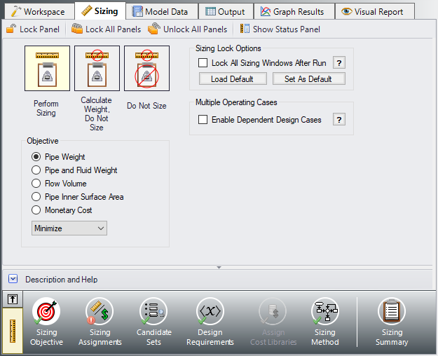
A. Sizing Objective
The Sizing Objective panel is used to set the Sizing Option, which is the type of calculation that will be performed, and to select an Objective which will be used in the sizing process.
For the Sizing Option, Perform Sizing should generally be selected, since this is the primary function of the ANS module. However, the other two options may be used for troubleshooting or informational purposes. For example, the Calculate Cost, Do Not Size option may be useful to calculate an initial cost for the system, or to verify your cost libraries. The Do Not Size option allows the model to be run normally in AFT Fathom without requiring any cost or sizing information. This is useful to preserve the information already entered in the Sizing window.
ØSelect Perform Sizing (if not already selected) to begin configuring the sizing settings.
Note: The Sizing Option can always be seen on the box on the left of the Sizing Navigation panel. Clicking this box will bring you to the Sizing Objective panel, where this status can be changed.
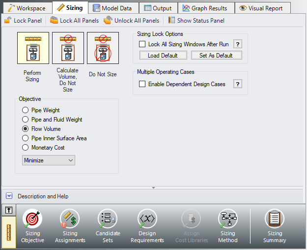
The easiest way to size the system is to set the objective to a non-monetary value such as pipe weight or flow volume rather than directly analyzing monetary cost. Here we will minimize flow volume. The flow volume is merely the sum of the internal volumes of all sized pipes. As the flow volume is minimized, the pipe material, and therefore cost, is minimized along with it. Typically it is recommended to use the pipe weight option, as this will have the best correlation to cost. However, certain systems, such as ducts may be better sized using flow volume.
Although we will not do so here, the ANS module can also minimize the monetary cost of the system. This is more powerful than sizing for flow volume, but also requires more time investment in setting up cost libraries.
ØFor the Objective, choose Flow Volume, and make sure Minimize is selected from the drop-down list. The Sizing Objective panel should now appear as shown in Figure 4.
B. Sizing Assignments
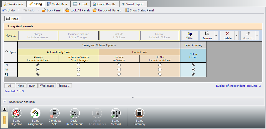
On the Sizing Navigation panel at the bottom of the window select the Sizing Assignments button. The Sizing Assignments panel allows the user to define what objects will be sized in the model, and what will be included in the cost calculation without being sized. Common Size Groups for pipes, or Maximum Cost Groups for pumps/control valves can be created on this panel as well when appropriate.
Let's consider the Sizing Assignments for the pipes, which should be displayed by default when we open this panel.
In the Sizing and Volume Options table there are several options under the categories to Automatically Size, or Do Not Size the pipe.
If an Automatically Size option is selected, the ANS module will treat the pipe diameter as a variable and vary it according to certain criteria that will be discussed shortly.
For a new system, typically all pipes will be desired to be sized and included in the cost, which is being calculated in terms of volume in this case. If you are instead analyzing the possible replacement of existing pipes, it may be better to size the pipes, but only include the cost if the size changes from that which exists.
If Do Not Size is selected, the pipe will retain the settings currently set in the Workspace. Why would one choose to not size a pipe? There could be a number of reasons, but one good reason is that the pipe represents a pipe in an existing system and the design does not allow the replacement of that pipe with a new one. Therefore its diameter is fixed, and sizing the pipe would serve no purpose.
Another reason may be if a certain size is necessary for the design due to certain requirements, in which case the pipe cost can be included without sizing the pipe by choosing Include in Cost.
This model is a new system, so all pipes will be sized and included in the cost.
ØSelect Always Include in Volume for all three pipes (Figure 5).
Since we want to size the pipes independently in this model, we do not need to make any changes to the Pipe Grouping section of the table, so this panel is complete.
Note: For models which have junctions that can be sized, a Junctions button at the top of this panel will be available to set the Junctions Sizing Assignments. In this case we have chosen to analyze flow volume. While this value can easily be calculated for the pipes, Fathom does not have enough information to calculate a flow volume for the branch or the reservoirs, which means that they cannot be sized using this method, and the Junctions tab is unavailable. This same limitation exists when using other non-monetary objectives as well, such as pipe weight. If the size of a junction will have a large impact on the system cost, such as a pump, Monetary Cost should be used as the Objective.
C. Candidate Sets
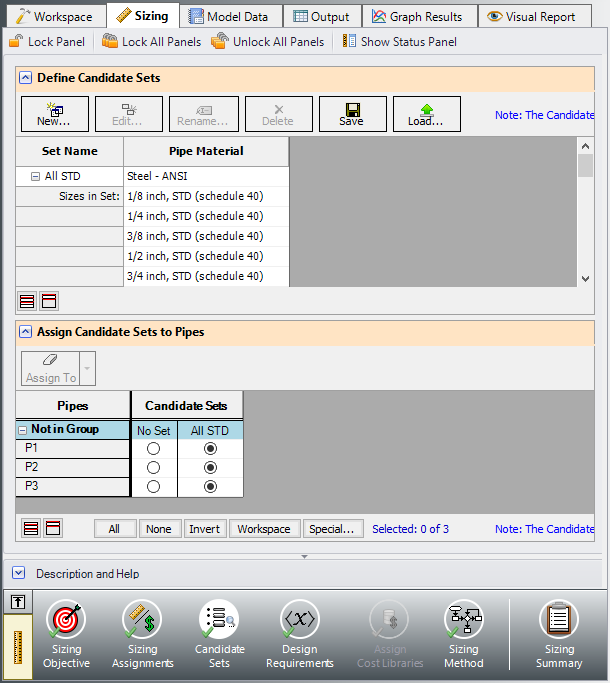
Click on the Candidate Sets button to open the Candidate Sets panel.
Since commercial piping is limited to certain sizes, the ANS module needs a list of possible sizes from which to choose. This list is called a Candidate Set.
So as not to limit the sizing unnecessarily, the candidate sets should include both smaller and larger pipes than your anticipated final size. If you make the candidate set too small, you may limit the ability of the ANS module to find the best sizing. It is better to make the candidate set too large than too small. Experience applying the ANS module to actual systems will help you choose appropriate candidate sets. If after obtaining a solution you find that one or more of the sized pipes is at the extreme of the candidate set a warning will appear, and it is recommended to expand the defined candidate set.
To create a Candidate Set, do the following:
-
Under Define Candidate Sets, click New.
-
Give the set the name All STD and click OK.
-
From the drop down list choose Steel - ANSI if it is not already selected.
-
At the bottom of the Select Pipe Sizes window, make sure the Sort option selection is Type, Schedule, Class.
-
In the Available Material Sizes and Types list on the left, select (not expand) STD so that the schedule name is now highlighted.
-
Click Add to add all STD pipe sizes to the list on the right.
-
Click OK.
The All STD set will now appear.
We will apply the All STD set shortly. First, let’s take a moment to understand what we have just done. We have created a candidate set that includes all pipe sizes in the library that are Steel - ANSI STD. At the low end this includes 1/8 inch pipe, and at the high end 48 inch pipe. This candidate set contains pipe sizes from a library of steel ANSI pipe, and not just specific pipes from the model. After we apply this candidate set to a specific pipe in the model and the sizing is run, the ANS module will select the best pipe size from this set of pipe sizes to achieve the objective.
We now need to define which pipes will use this Candidate Set during the sizing calculation. Each pipe that is being sized must have a Candidate Set assigned to it. Under Assign Candidate Sets to Pipes, set each pipe in the model to use All STD by selecting the radio button under this candidate set for each of the pipes. The Candidate Sets should now be fully defined and assigned to the appropriate pipes, as can be seen in Figure 6.
D. Design Requirements
Select the Design Requirements button. If we do not define any design requirements for the model, the ANS module will automatically choose the smallest pipe size in the Candidate Set, since it has the smallest flow volume. Along with the smallest pipes we may get unacceptably low flow rates, or unacceptably high velocities and pressure drops. To maintain acceptable system operating conditions, we need to set design requirements.
We are going to define two design requirements for this case. Before adding any requirements, let’s look more closely at the results of the model we are starting with. All pipe diameters are nominal 8 inch, and the results show that the water flows from reservoir J1 to reservoirs J2 and J3. The flowrate out of J1 is
We need to create two Design Requirements that represent the flow requirements at the reservoirs in order to answer this question. We will do this by defining Design Requirements for the inlet/outlet flowrates of the pipes where they connect to each of the Reservoirs. To do this:
-
Make sure that the Pipes button is selected.
-
Click New under Define Design Requirements.
-
Enter a name when prompted: Min Flow Supply. Click OK.
-
A new row will appear in the Pipe Design Requirements table. In this row, select Volumetric Flow Rate as the Parameter.
-
Choose Minimum for Max/Min.
-
Enter 2500 gal/min.
-
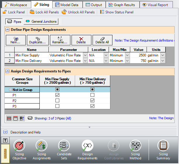
Now repeat the above process to define Min Flow Delivery with a Volumetric Flow Rate Minimum of 750 gal/min.
To be functional, we need to apply these Design Requirements to the correct pipes. There are no limits to the number of Design Requirements that can be defined and applied.
In the Assign Design Requirements to Pipes section, expand the pipe list. Select the check box for Min Flow Supply next to pipe P1, and Min Flow Delivery next to pipes P2 and P3. This will set the minimum flow rate coming out of Reservoir J1 and going into Reservoirs J2 and J3 as described above. The fully defined and assigned Design Requirements are shown in Figure 7.
E. Assign Cost Libraries
When the Sizing Objective has been defined as Monetary Cost, it is necessary to create and assign cost libraries for the automated sizing, which can be done in the Assign Cost Libraries panel. Since we have defined the objective as Pipe Flow Volume, we will not need to assign any cost libraries, and this button is grayed out.
F. Sizing Method
Select the Sizing Method button to go to the Sizing Method panel.
The Sizing Method panel is used to set up the calculation methods for sizing the system. You can select whether discrete or continuous sizing will be used, and which method will be applied.
If Continuous Sizing is selected, the ANS module will ignore the defined Candidate Sets and report the ideal hydraulic diameter for the pipes being sized, which will likely not match any of the possible chosen commercial sizes. While this is not useful as a final solution, this may be helpful as a baseline to check the final solution using the provided discrete methods. Discrete Sizing will typically perform a continuous sizing calculation as a basis, after which multiple discrete sizes above and below this solution will be evaluated to find the ideal sizing based on the provided Candidate Set.
ØFor this model, use Discrete Sizing.
For the Search Method, the ideal method will often change based on the number of independent pipe sizes (shown in the Sizing Assignments panel on the bottom right), number of Design Requirements, and feasibility of the initial system design. The Help file provides more information on the strengths and weaknesses of each method. It is generally recommended to run the sizing with more than one method, as it is often not obvious which method will be most effective for each system. The suggest Method button can be used as a guide for which method to start with.
For a simple model such as this one, the MMFD or SQP method should be appropriate since there are only a few Design Requirements, and only three pipes are being varied.
ØChoose the default Modified Method of Feasible Directions (MMFD).
Step 5. Run the Model
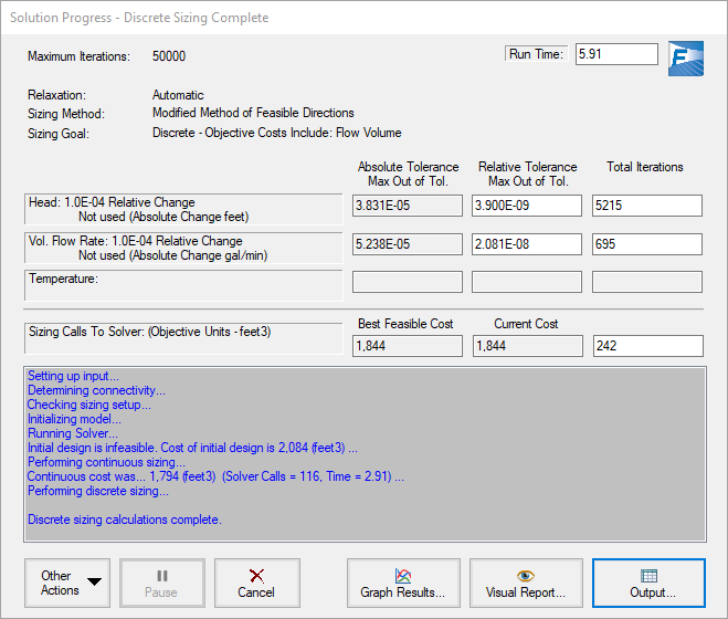
Select Run from the Analysis menu. While the model is running, the Solution Progress window shows the Sizing Calls to Solver. This is how many times a complete hydraulic analysis was run.
The solver also displays the Current Cost and Best Feasible Cost, which will display the last calculated value for the cost, as well as the Best Feasible Cost which has been found so far (Figure 8). The solver will continue to iterate using the defined method until it finds the ideal sizing. For the selected method, the solver will first perform a continuous sizing to find a starting point, then test discrete solutions close to this continuous solution to find the final, discrete solution.
Note: At any time during the run, the user can pause the solution and use the Other Actions button to accept the currently displayed Best Feasible Cost as the final solution. For this example the solution is found and displayed quickly, but for larger systems with many pipes being sized, it may be more productive to pause the solution and accept the current solution in order to save time, especially if the displayed cost does not appear to be decreasing much further.
Step 6. Review the Sized Results
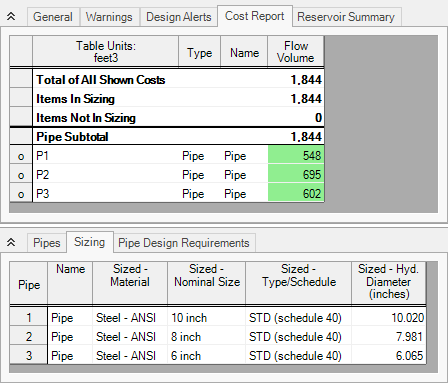
Click the View Output button to see the results. The General section shows the Cost Report, which indicates the volumes for the final solution. As shown in Figure 9, the minimum total volume identified by the ANS module was
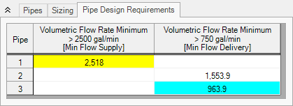
Now switch to the Pipe Design Requirements tab in the Pipe section (Figure 10). We can confirm that the calculated design is feasible, since all of the Design Requirements were met. That is, the flow from J1 (as shown in pipe P1) exceeded
You can also display the adjusted pipe sizes and resulting flow rates in the Visual Report.
When performing sizing, the Transfer Results to Initial Guesses feature on the Output window Edit menu takes on new meaning. When used in a non-sizing context, this feature takes the solved hydraulic results (i.e., pressures, flows rates, etc.) and assigns them to the initial guess values for the pipes and junctions.
When you select Transfer Results to Initial Guesses after automated sizing, you will see a dialog window appear like that shown in Figure 11. The ANS module allows you to transfer the hydraulic results, the sized pipe diameters, or both. If you transfer the sized pipe diameters, each pipe's input diameter (back on the Workspace) will become the sized diameter.
This feature allows the sizing results to be saved to the model for use in further analysis as needed.
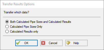
Figure 11: After sizing, the Transfer Results to Initial Guesses feature transfers both the hydraulic results and sized pipe size results
Conclusion
You have now used performed a network sizing to minimize flow volume with the ANS module.


