Cooling System (English Units)
Summary
The objective of this example is to determine how much flow will be delivered to the heat exchangers in the system. A secondary objective is to determine the best pump for the system.
Topics Covered
-
Modeling a closed loop system
-
Using a pressure reducing valve
-
Generating a pump curve
-
Generating a resistance curve for a heat exchanger
-
Importing a pump curve to obtain pump data
Required Knowledge
This example assumes the user has already worked through the Beginner: Three Reservoir Problem example, or has a level of knowledge consistent with that topic. You can also watch the AFT Fathom Quick Start Video Tutorial Series on the AFT website, as it covers the majority of the topics discussed in the Three-Reservoir Problem example.
Model Files
This example uses the following files, which are installed in the Examples folder as part of the AFT Fathom installation:
Note: If you open the completed US - Cooling System.fth model file, you will notice a child scenario named Initial Model for ANS Quick Start Chapter 3. This child scenario is used as the starting point for a model in the ANS Quick Start Guide. This scenario can be disregarded when comparing your model to this completed model.
Step 1. Start AFT Fathom
From the Start Menu choose the AFT Fathom 12 folder and select AFT Fathom 12.
To ensure that your results are the same as those presented in this documentation, this example should be run using all default AFT Fathom settings, unless you are specifically instructed to do otherwise.
Step 2. Define the Fluid Properties Group
-
Open Analysis Setup from the toolbar or from the Analysis menu.
-
Open the Fluid panel then define the fluid:
-
Fluid Library = AFT Standard
-
Fluid = Dowtherm J (after selecting, click Add to Model)
-
Temperature = 150 deg. F
-
Step 3. Define the Pipes and Junctions Group
At this point, the first two groups are completed in Analysis Setup. The next undefined group is the Pipes and Junctions group. To define this group, the model needs to be assembled with all pipes and junctions fully defined. Click OK to save and exit Analysis Setup then assemble the model on the workspace as shown in the figure below.
To add the segment into pipe P22, use the Pipe Segments tool on the Arrange menu.
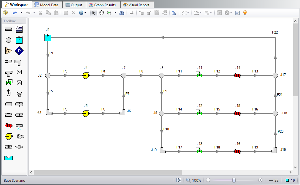
Figure 1: Workspace window for Cooling System Problem
Pipe Properties
-
Pipe Model tab
-
Pipe Material = Steel - ANSI
-
Pipe Geometry = Cylindrical Pipe
-
Size = Use table below
-
Type = STD (schedule 40)
-
Friction Model Data Set = Standard
-
Lengths = Use table below
-
| Pipe | Size | Length (feet) |
|---|---|---|
| 1 | 6 inch | 20 |
| 2, 7, 9-10, 20-21 | 4 inch | 3 |
| 3-6, 12-13, 15-16, 18-19 | 4 inch | 5 |
| 11, 14, 17 | 4 inch | 10 |
| 8, 22 | 6 inch | 200 |
Junction Properties
-
J1 Reservoir
-
Liquid Surface Elevation = 10 feet
-
Liquid Surface Pressure = 40 psig
-
Pipe Depth = 10 feet
-
-
All Branches
-
Elevation = 2 feet
-
-
All Bends
-
Inlet Elevation = 2 feet
-
Type = Standard Elbow (knee, threaded)
-
Angle = 90 Degrees
-
-
J4 & J5 Pumps
-
Inlet Elevation = 2 feet
-
Pump Model = Centrifugal (Rotodynamic)
-
Analysis Type = Pump Curve
-
Enter Curve Data =
-
| Volumetric | Head |
|---|---|
| gal/min | feet |
| 0 | 70 |
| 500 | 60 |
| 1000 | 40 |
-
Curve Fit Order = 2
-
All Control Valves
-
Inlet Elevation = 2 feet
-
Valve Type = Pressure Reducing (PRV)
-
Control Setpoint = Pressure, Static
-
Setpoint = 50 psig
-
-
All Heat Exchangers
-
Inlet Elevation = 2 feet
-
Loss Model = Resistance Curve
-
Enter Curve Data =
-
| Volumetric | Pressure |
|---|---|
| gal/min | psid |
| 500 | 10 |
-
Click Fill As Quadratic
-
Curve Fit Order = 2
ØTurn on Show Object Status from the View menu to verify if all data is entered. If so, the Pipes and Junctions group in Analysis Setup will have a check mark. If not, the uncompleted pipes or junctions will have their number shown in red. If this happens, go back to the uncompleted pipes or junctions and enter the missing data.
Step 4. Run the Model
Click Run Model on the toolbar or from the Analysis menu. This will open the Solution Progress window. This window allows you to watch as the AFT Fathom solver converges on the answer. This model runs very quickly. Now view the results by clicking the Output button at the bottom of the Solution Progress window.
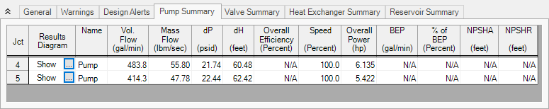
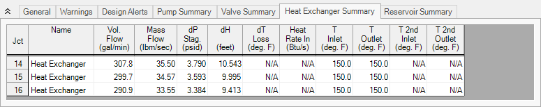
Step 5. Examine the Output
The output is shown below in Figure 2. The pump summary shows that the head requirement for the pumps is
Step 6. Evaluate Other Pumps
The customer for this project wants an evaluation of three other pumps to determine which uses the least energy. The pump curve for each of these pumps is found in a text file.
For each of the pumps follow the following set of steps:
-
Create a child of the base scenario in the Scenario Manager on the Quick Access Panel for Pump A, Pump B, and Pump C.
-
Load scenario Pump A, open the Pump Properties window, click Enter Curve Data
-
Click Edit Table and select Import From File
-
Change the file format to Text (*.txt) then select the data file US - Cooling System Pump A.txt and click Open.
-
Using the Comma Separator, click OK.
-
With a Curve Fit Order of 2, click Generate Curve Fit Now, then click OK
-
Select the second pump and set all the properties equal to the first pump.
Run each scenario and take note of the overall pump power in the pump summary window. The data should match the following:
|
|
J4 | J5 |
|---|---|---|
| A | 5.755 hp | 4.509 hp |
| B | 6.866 hp | 5.489 hp |
| C | 6.546 hp | 4.403 hp |
From this data, Pump A is the best choice, because it consumes the least power.


