Crude Oil Pipeline (Metric Units)

Summary

The objective of this example is to model a pipeline system to investigate the effects of a viscous fluid. We will answer a number of questions about the pipeline system such as:

1. How does viscosity affect pump performance?

2. What is the flow rate?

3. What is the maximum pressure in the pipe?

4. Is the flow laminar or turbulent?

5. How high can the hill be until a vacuum (i.e., less than atmospheric pressure) is created?

6. How does the hill height affect flow rate?

7. How much can the pump speed be slowed down and still not pull a vacuum?

Required Knowledge

This example assumes the user has already worked through the Beginner: Three Reservoir Problem example, or has a level of knowledge consistent with that topic. You can also watch the AFT Fathom Quick Start Video Tutorial Series on the AFT website, as it covers the majority of the topics discussed in the Three-Reservoir Problem example.

Model File

This example uses the following file, which is installed in the Examples folder as part of the AFT Fathom installation:

• US - Crude Oil Pipeline.fth

Step 1. Start AFT Fathom

From the Start Menu choose the AFT Fathom 12 folder and select AFT Fathom 12.

To ensure that your results are the same as those presented in this documentation, this example should be run using all default AFT Fathom settings, unless you are specifically instructed to do otherwise.

Step 2. Define the Fluid Properties Group

1. Open Analysis Setup from the toolbar or from the Analysis menu.

2. Open the Fluid panel then define the fluid:

   1. Fluid Library = User Specified Fluid

   2. Name = Petroleum Product

   3. Density = 0.8 S.G. water

   4. Dynamic Viscosity = 500 centipoise

Step 3. Define the Pipes and Junctions Group

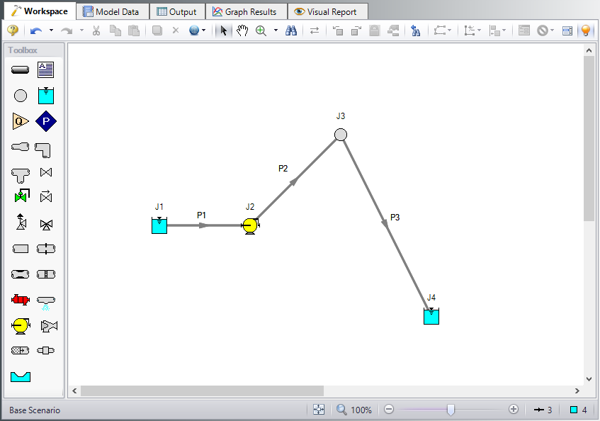
At this point, the first two groups are completed in Analysis Setup. The next undefined group is the Pipes and Junctions group. To define this group, the model needs to be assembled with all pipes and junctions fully defined. Click OK to save and exit Analysis Setup then assemble the model on the workspace as shown in the figure below.

Pipe Properties

1. Pipe Model tab

   1. Pipe Material = Steel - ANSI

   2. Pipe Geometry = Cylindrical Pipe

   3. Size = 24 inch

   4. Type = STD (schedule 20)

   5. Friction Model Data Set = Standard

   6. Lengths =

Pipe	Length
1	100 feet
2	25 miles
3	50 miles

Junction Properties

Enter the properties of the junctions in the workspace as follows:

1. J1 Reservoir

   1. Liquid Surface Elevation = 750 feet

   2. Liquid Surface Pressure = 0 psig

   3. Pipe Depth = 10 feet

2. J2 Pump

   1. Inlet Elevation = 720 feet

   2. Pump Model = Centrifugal (Rotodynamic)

   3. Analysis Type = Pump Curve

   4. Enter Curve Data =

Volumetric	Head
barrels/day	feet
0	2000
100,000	1800
200,000	1400

5. Curve Fit Order = 2

 Note: If barrels/day is not an available unit, select User Options from the Tools menu, click on Preferred Units, and select the radio button for All Units.

4. J3 Branch

   1. Elevation = 1250 feet

5. J4 Reservoir

   1. Liquid Surface Elevation = 10 feet

   2. Liquid Surface Pressure = 0 psig

   3. Pipe Depth = 10 feet

In the Pump Properties window on the Optional tab, Fathom includes an option to Use Viscosity Correction.  We will turn this option on later to determine how much this option affects the answers. Leave the option off for now.

ØTurn on Show Object Status from the View menu to verify if all data is entered. If so, the Pipes and Junctions group in Analysis Setup will have a check mark. If not, the uncompleted pipes or junctions will have their number shown in red. If this happens, go back to the uncompleted pipes or junctions and enter the missing data.

Step 4. Run the Model

Click Run Model on the toolbar or from the Analysis menu. This will open the Solution Progress window. This window allows you to watch as the AFT Fathom solver converges on the answer. This model runs very quickly. Now view the results by clicking the Output button at the bottom of the Solution Progress window.

Step 5. Examine the Output

Open the Output Control window by selecting Output Control from the toolbar or Tools menu. On the Display Parameters tab, select the Pumps button to display the list of output parameters that are specific to pumps. Then add the three correction parameters to pump efficiency CE, pump head rise CH, and pump flow CQ.  These are the pump viscosity correction/pump de-rating factors that will de-rate the pump according to the Hydraulic Institute method, ANSI/HI Standard 9.6.7-2010. Change the Volumetric Flow Rate units to barrels/day.

Now select the Pipes button to display the pipe output parameters, then change the units for Volumetric Flow Rate to barrels/day. Also, add Reynolds Number to the list of output variables. Click OK to save the changes and close Output Control.

The Output window contains all the data that was specified in the output control window. The output from this model is shown in Figure 2. Note that the flow rate in all the pipes is 151,571 barrels/day.

Return to the workspace and open the pump properties window. Navigate to the Optional tab and check the box for Use Viscosity Correction. Input the following:

1. Head Correction (ANSI/HI 9.6.7-2015) = Assume Calculated Flow Is At BEP

2. Rated Speed (rpm) = 3600

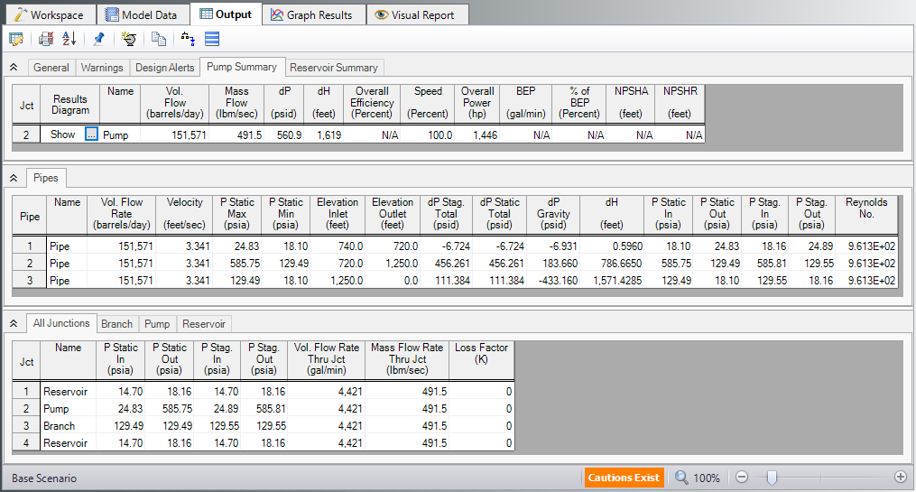
Click OK and run the model again. The output from this run is shown below. Now notice that the flow rate is 143,822 barrels/day. Click the Pump Summary tab in the General Output section to see the values for CE, CH, and CQ. The output from this model is shown in Figure 3.

Question 1. How does viscosity affect pump performance?

The flow rate, pump head, and overall power all decreased when the viscosity corrections were used.

Question 2. What is the flow rate?

Before the viscosity correction was added the flow rate was 151,571 barrels/day. After the viscosity correction was added the flow rate became 143,822 barrels/day. Therefore, the viscosity correction factor reduced the flow rate by approximately 5.1%.

Question 3. What is the maximum pressure in the pipe?

The maximum pressure can be found in the pipe summary in the P Static Max column. It occurs in Pipe 2 and it occurs at the inlet of the pipe (outlet of the pump). The pressure is 543.93 psia or 529.24 psig.

Question 4. Is the flow laminar or turbulent?

In the pipe summary window we can see that the Reynolds number is 912.2. Therefore the flow is laminar. The general cut-off for laminar flow is Reynolds number greater than 2,300.

Question 5. How high can the hill be until a vacuum is created?

To answer this question we have to change the elevation of branch J3 and re-run the model. If the hill height is raised to 1500 feet, the minimum pressure in pipe 2 and 3 and at junction J3 is 14.98 psia, or nearly atmospheric pressure. If the hill is higher than 1500 feet, a vacuum would be created. This output can be seen in Figure 4.

Question 6. How does the hill height affect flow rate?

Compare Figure 3 and Figure 4 and you will see that the flow rate is exactly the same. Because the pipe length is the same and the net elevation change is the same, the flow rate will be the same.

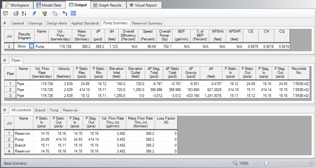
Question 7. How much can the pump speed be slowed down and still not pull a vacuum?

The pump can be slowed down to 86.6% before the minimum pressure in pipes 2 and 3 goes below atmospheric (14.7 psia). The output of this run is shown in Figure 5.